AMath 483/583 Lecture 27 Notes: Outline: Random walk solution of - - PDF document

AMath 483/583 — Lecture 27

Outline:

• Random walk solution of Poisson problem
• Using MPI with subroutines
• Python plus Fortran: f2py

Notes and Sample codes:

• Class notes: Random numbers
• Class notes: Poisson problem
• $UWHPSC/codes/mpi/quadrature
• $UWHPSC/codes/f2py

R.J. LeVeque, University of Washington AMath 483/583, Lecture 27

Notes:

R.J. LeVeque, University of Washington AMath 483/583, Lecture 27

Monte Carlo solution of Poisson problem

Suppose we want to compute an approximate solution to uxx + uyy = 0 with u given on boundary at a single point (x0, y0). Finite difference approach: Discretize domain and solve linear system for approximations Uij at all points on grid. Instead can take a random walk starting at (x0, y0) and evaluate u at the first boundary point the walk reaches. Do this N times and average all the values obtained. This average converges to u(x0, y0) with rate 1/ √ N.

R.J. LeVeque, University of Washington AMath 483/583, Lecture 27

Notes:

R.J. LeVeque, University of Washington AMath 483/583, Lecture 27

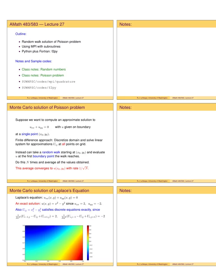
Monte Carlo solution of Laplace’s Equation

Laplace’s equation: uxx(x, y) + uyy(x, y) = 0 An exact solution: u(x, y) = x2 − y2 since uxx = 2, uyy = −2. Also Uij = x2

i − y2 j satisfies discrete equations exactly, since 1 ∆x2 (Ui−1,j − Uij + Ui+1,j) = 2, 1 ∆y2 (Ui,j−1 − Uij + Ui,j+1) = −2

R.J. LeVeque, University of Washington AMath 483/583, Lecture 27

Notes:

R.J. LeVeque, University of Washington AMath 483/583, Lecture 27

Random walk on a lattice

uxx + uyy = 0 with solution u(x, y) = x2 − y2. Estimate solution at (x0, y0) = (0.9, 0.6) where u(x0, y0) = 0.45.

R.J. LeVeque, University of Washington AMath 483/583, Lecture 27

Notes:

R.J. LeVeque, University of Washington AMath 483/583, Lecture 27

Random walk on a lattice

Strategy: Start at (x0, y0). Each step, move to one of 4 neighbors, choosing with equal probability. If 0 ≤ r ≤ 1 is a uniformly distributed random number then decide based on: 0 ≤ r < 0.25 = ⇒ move left 0.25 ≤ r < 0.5 = ⇒ move right 0.5 ≤ r < 0.75 = ⇒ move down 0.75 ≤ r ≤ 1.0 = ⇒ move down

R.J. LeVeque, University of Washington AMath 483/583, Lecture 27

Notes:

R.J. LeVeque, University of Washington AMath 483/583, Lecture 27

Random walk on a lattice

Why does this work? Let Eij be expected value of boundary value reached if starting at grid point (i, j). Then Eij = 1

4(Ei−1,j + Ei+1,j + Ei,j−1 + Ei,j+1)

The same equation as finite difference method for Poisson!

R.J. LeVeque, University of Washington AMath 483/583, Lecture 27

Notes:

R.J. LeVeque, University of Washington AMath 483/583, Lecture 27

MPI with subroutines and functions

Recall quadrature program from Homework 4: In OpenMP: Subroutine is called by the single master thread running the main program Inside the subroutine trapezoid a single omp parallel block is used to fork a set of threads that are used for the full computation. End of a parallel block kills all threads except master thread. In MPI: First statement in main program must be MPI_INIT. It’s not possible to call MPI_INIT in the subroutine. The entire code (including main program and call to subroutine) is executed by each process (maybe on different computers!). Call to MPI_FINALIZE kills all processes.

R.J. LeVeque, University of Washington AMath 483/583, Lecture 27

Notes:

R.J. LeVeque, University of Washington AMath 483/583, Lecture 27

MPI with subroutines and functions

MPI version of Simpson’s rule program: $UWHPSC/codes/mpi/quadrature Notes:

• There is no master process except that we may decide

some things should only be done by Process 0, for example.

• The module variable gevals is a global variable, but is still

private to each process. All variables are private, no shared variables!

R.J. LeVeque, University of Washington AMath 483/583, Lecture 27

Notes:

R.J. LeVeque, University of Washington AMath 483/583, Lecture 27

f2py — combining Fortran and Python

Often want to use Fortran for intensive computations, Python to provide nice user interface, plot results, automate a series of runs with different parameters, do convergence tests as grid size is refined, etc. Can write data files to disk from Fortran, read into Python, This is what we’ve done for plotting in homeworks. Sometimes nice to call Fortran directly from Python. e.g. LAPACK is used under the hood in NumPy. f2py provides a wrapper for Fortran code.

R.J. LeVeque, University of Washington AMath 483/583, Lecture 27

Notes:

R.J. LeVeque, University of Washington AMath 483/583, Lecture 27

f2py — combining Fortran and Python

Basic idea: fortrancode.f90 contains a function or subroutine, e.g. function f1(x) that returns a single value. $ f2py -m mymodulename -c fortrancode.f90 This creates a binary file mymodulename.so that can used as a Python module. >>> from mymodulename import f1 >>> y = f1(3.)

R.J. LeVeque, University of Washington AMath 483/583, Lecture 27

Notes:

R.J. LeVeque, University of Washington AMath 483/583, Lecture 27

f2py — function example

$UWHPSC/codes/f2py/fcn1.f90 function f1(x) real(kind=8), intent(in) :: x real(kind=8) :: f1 f1 = exp(x) end function f1 Then we can do... $ f2py -m fcn1 -c fcn1.f90 $ python >>> import fcn1 >>> fcn1.f1(1.) 2.7182818284590451

R.J. LeVeque, University of Washington AMath 483/583, Lecture 27

Notes:

R.J. LeVeque, University of Washington AMath 483/583, Lecture 27

f2py — subroutine example

$UWHPSC/codes/f2py/sub1.f90 subroutine mysub(a,b,c,d) real (kind=8), intent(in) :: a,b real (kind=8), intent(out) :: c,d c = a+b d = a-b end subroutine mysub Then we can do... $ f2py -m sub1 -c sub1.f90 $ python >>> import sub1 >>> y = sub1.mysub(3., 5.) >>> print y (8.0, -2.0) Note: Tuple (c, d) is returned by the Python function.

R.J. LeVeque, University of Washington AMath 483/583, Lecture 27

Notes:

R.J. LeVeque, University of Washington AMath 483/583, Lecture 27

f2py — Jacobi iteration

$UWHPSC/codes/f2py/jacobi1.f90 subroutine iterate(u0,iters,f,u,n) Takes input array u0 of length n and right hand side array f and produces u by taking iters iterations of Jacobi. $UWHPSC/codes/f2py/plot_jacobi_iterates.py # Set u = initial guess; f = rhs for nn in range(nplots): u = jacobi1.iterate(u, iters_per_plot, f) plt.plot(x, u, ’o-’) plt.draw() time.sleep(.5)

R.J. LeVeque, University of Washington AMath 483/583, Lecture 27

Notes:

R.J. LeVeque, University of Washington AMath 483/583, Lecture 27

Other wrappers...

• Cython: Allows writing C code embedded in Python.

http://www.cython.org/

• Jython: For Java.

http://www.jython.org/

• swig: Connects C and C++ to many other languages

http://www.swig.org/

R.J. LeVeque, University of Washington AMath 483/583, Lecture 27

Notes:

R.J. LeVeque, University of Washington AMath 483/583, Lecture 27