AMath 483/583 Lecture 24 Notes: Outline: Heat equation and - PDF document

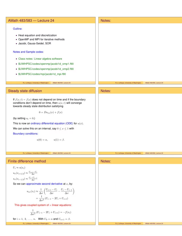
AMath 483/583 — Lecture 24 Notes: Outline: • Heat equation and discretization • OpenMP and MPI for iterative methods • Jacobi, Gauss-Seidel, SOR Notes and Sample codes: • Class notes: Linear algebra software • $UWHPSC/codes/openmp/jacobi1d_omp1.f90 • $UWHPSC/codes/openmp/jacobi1d_omp2.f90 • $UWHPSC/codes/mpi/jacobi1d_mpi.f90 R.J. LeVeque, University of Washington AMath 483/583, Lecture 24 R.J. LeVeque, University of Washington AMath 483/583, Lecture 24 Steady state diffusion Notes: If f ( x, t ) = f ( x ) does not depend on time and if the boundary conditions don’t depend on time, then u ( x, t ) will converge towards steady state distribution satisfying 0 = Du xx ( x ) + f ( x ) (by setting u t = 0 .) This is now an ordinary differential equation (ODE) for u ( x ) . We can solve this on an interval, say 0 ≤ x ≤ 1 with Boundary conditions: u (0) = α, u (1) = β. R.J. LeVeque, University of Washington AMath 483/583, Lecture 24 R.J. LeVeque, University of Washington AMath 483/583, Lecture 24 Finite difference method Notes: U i ≈ u ( x i ) u x ( x i +1 / 2 ) ≈ U i +1 − U i ∆ x u x ( x i − 1 / 2 ) ≈ U i − U i − 1 ∆ x So we can approximate second derivative at x i by: 1 � U i +1 − U i � − U i − U i − 1 u xx ( x i ) ≈ ∆ x ∆ x ∆ x 1 = ∆ x 2 ( U i − 1 − 2 U i + U i +1 ) This gives coupled system of n linear equations: 1 ∆ x 2 ( U i − 1 − 2 U i + U i +1 ) = − f ( x i ) for i = 1 , 2 , . . . , n . With U 0 = α and U n +1 = β . R.J. LeVeque, University of Washington AMath 483/583, Lecture 24 R.J. LeVeque, University of Washington AMath 483/583, Lecture 24

Iterative methods Notes: Coupled system of n linear equations: ( U i − 1 − 2 U i + U i +1 ) = − ∆ x 2 f ( x i ) for i = 1 , 2 , . . . , n . With U 0 = α and U n +1 = β . Iterative method starts with initial guess U [0] to solution and then improves U [ k ] to get U [ k +1] for k = 0 , 1 , . . . . Note: Generally does not involve modifying matrix A . Do not have to store matrix A at all, only know about stencil. R.J. LeVeque, University of Washington AMath 483/583, Lecture 24 R.J. LeVeque, University of Washington AMath 483/583, Lecture 24 Jacobi iteration Notes: ( U i − 1 − 2 U i + U i +1 ) = − ∆ x 2 f ( x i ) Solve for U i : U i = 1 U i − 1 + U i +1 + ∆ x 2 f ( x i ) � � . 2 Note: With no heat source, f ( x ) = 0 , the temperature at each point is average of neighbors. Suppose U [ k ] is a approximation to solution. Set = 1 U [ k +1] � U [ k ] i − 1 + U [ k ] � i +1 + ∆ x 2 f ( x i ) for i = 1 , 2 , . . . , n. i 2 Repeat for k = 0 , 1 , 2 , . . . until convergence. Can be shown to converge (eventually... very slow!) R.J. LeVeque, University of Washington AMath 483/583, Lecture 24 R.J. LeVeque, University of Washington AMath 483/583, Lecture 24 Jacobi iteration in Fortran Notes: uold = u ! starting values before updating do iter=1,maxiter dumax = 0.d0 do i=1,n u(i) = 0.5d0*(uold(i-1) + uold(i+1) + dx**2*f(i)) dumax = max(dumax, abs(u(i)-uold(i))) enddo ! check for convergence: if (dumax .lt. tol) exit uold = u ! for next iteration enddo Note: we must use old value at i − 1 for Jacobi. Otherwise we get the Gauss-Seidel method. u(i) = 0.5d0*(u(i-1) + u(i+1) + dx**2*f(i)) This actually converges faster! R.J. LeVeque, University of Washington AMath 483/583, Lecture 24 R.J. LeVeque, University of Washington AMath 483/583, Lecture 24

Jacobi with OpenMP – coarse grain Notes: General Approach: • Fork threads only once at start of program. • Each thread is responsible for some portion of the arrays, from i=istart to i=iend . • Each iteration, must copy u to uold , update u , check for convergence. • Convergence check requires coordination between threads to get global dumax . • Print out final result after leaving parallel block See code in the repository or the notes: $UWHPSC/codes/openmp/jacobi1d_omp2.f90 R.J. LeVeque, University of Washington AMath 483/583, Lecture 24 R.J. LeVeque, University of Washington AMath 483/583, Lecture 24 Jacobi with MPI Notes: Each process is responsible for some portion of the arrays, from i=istart to i=iend . No shared memory: each process only has part of array. Updating formula: u(i) = 0.5d0*(uold(i-1) + uold(i+1) + dx**2*f(i)) Need to exchange values at boundaries: Updating at i=istart requires uold(istart-1) Updating at i=iend requires uold(istart+1) Example with n = 9 interior points (plus boundaries): Process 0 has istart = 1, iend = 5 Process 1 has istart = 6, iend = 9 R.J. LeVeque, University of Washington AMath 483/583, Lecture 24 R.J. LeVeque, University of Washington AMath 483/583, Lecture 24 Jacobi with MPI — Sending to neighbors Notes: call mpi_comm_rank(MPI_COMM_WORLD, me, ierr) ... do iter = 1, maxiter uold = u if (me > 0) then ! Send left endpoint value to "left" call mpi_isend(uold(istart), 1, MPI_DOUBLE_PRECISION, me - 1, 1, MPI_COMM_WORLD, req1, ierr) end if if (me < ntasks-1) then ! Send right endpoint value to "right" call mpi_isend(uold(iend), 1, MPI_DOUBLE_PRECISION, me + 1, 2, MPI_COMM_WORLD, req2, ierr) end if end do Note: Non-blocking mpi_isend is used, Different tags (1 and 2) for left-going, right-going messages. R.J. LeVeque, University of Washington AMath 483/583, Lecture 24 R.J. LeVeque, University of Washington AMath 483/583, Lecture 24

Jacobi with MPI — Receiving from neighbors Notes: Note: uold(istart) from me+1 goes into uold(iend+1) : uold(iend) from me-1 goes into uold(istart-1) : do iter = 1, maxiter ! mpi_send’s from previous slide if (me < ntasks-1) then ! Receive right endpoint value call mpi_recv(uold(iend+1), 1, MPI_DOUBLE_PRECISION, me + 1, 1, MPI_COMM_WORLD, mpistatus, ierr) end if if (me > 0) then ! Receive left endpoint value call mpi_recv(uold(istart-1), 1, MPI_DOUBLE_PRECISION, me - 1, 2, MPI_COMM_WORLD, mpistatus, ierr) end if ! Apply Jacobi iteration on my section of array do i = istart, iend u(i) = 0.5d0*(uold(i-1) + uold(i+1) + dx**2*f(i)) dumax_task = max(dumax_task, abs(u(i) - uold(i))) end do end do R.J. LeVeque, University of Washington AMath 483/583, Lecture 24 R.J. LeVeque, University of Washington AMath 483/583, Lecture 24 Jacobi with MPI Notes: Other issues: • Convergence check requires coordination between processes to get global dumax . Use MPI_ALLREDUCE so all process check same value. • Part of final result must be printed by each process (into common file heatsoln.txt ), in proper order. See code in the repository or the notes: $UWHPSC/codes/mpi/jacobi1d_mpi.f90 R.J. LeVeque, University of Washington AMath 483/583, Lecture 24 R.J. LeVeque, University of Washington AMath 483/583, Lecture 24 Jacobi with MPI — Writing solution in order Notes: Want to write table of values x(i),u(i) in heatsoln.txt . Need them to be in proper order, so Process 0 must write to this file first, then Process 1, etc. Approach: Each process me waits for a message from me-1 indicating that it has finished writing its part. (Contents not important.) Each process must open the file (without clobbering values already there), write to it, then close the file. Assumes all processes share a file system! On cluster or supercomputer, need to either: send all results to single process for writing, or write distributed files that may need to be combined later (some visualization tools handle distributed data!) R.J. LeVeque, University of Washington AMath 483/583, Lecture 24 R.J. LeVeque, University of Washington AMath 483/583, Lecture 24

Jacobi in 2D Notes: Updating point 7 for example ( u 32 ): = 1 U [ k +1] 4( U [ k ] 22 + U [ k ] 42 + U [ k ] 21 + U [ k ] 41 + h 2 f 32 ) 32 R.J. LeVeque, University of Washington AMath 483/583, Lecture 24 R.J. LeVeque, University of Washington AMath 483/583, Lecture 24 Jacobi in 2D using MPI Notes: With two processes: Could partition unknown into Process 0 takes grid points 1–8 Process 1 takes grid points 9–16 Each time step: Process 0 sends top boundary (5–8) to Process 1, Process 1 sends bottom boundary (9–12) to Process 0. R.J. LeVeque, University of Washington AMath 483/583, Lecture 24 R.J. LeVeque, University of Washington AMath 483/583, Lecture 24 Jacobi in 2D using MPI Notes: With more grid points and processes... Could partition several different ways, e.g. with 4 processes: The partition on the right requires less communication. With m 2 processes on grid with n 2 points: 2( m 2 − 1) n boundary points on left, 4( m − 1) n boundary points on right. R.J. LeVeque, University of Washington AMath 483/583, Lecture 24 R.J. LeVeque, University of Washington AMath 483/583, Lecture 24