AMath 483/583 Lecture 12 Notes: Outline: More about computer - PDF document

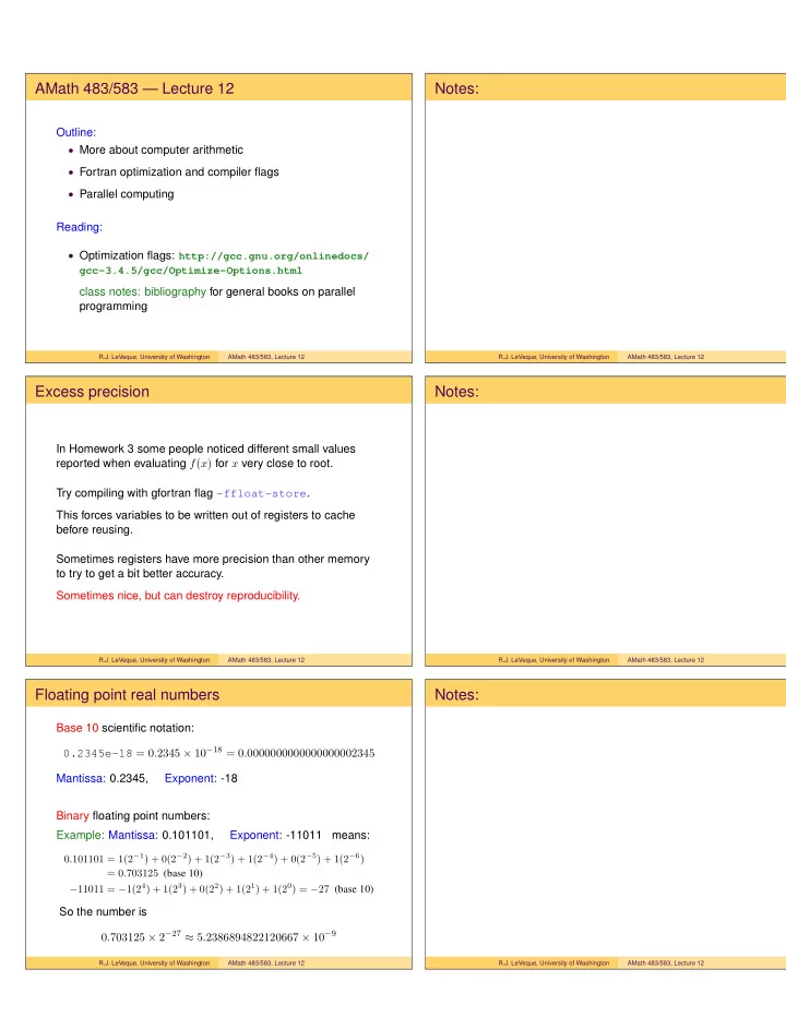
AMath 483/583 — Lecture 12 Notes: Outline: • More about computer arithmetic • Fortran optimization and compiler flags • Parallel computing Reading: • Optimization flags: http://gcc.gnu.org/onlinedocs/ gcc-3.4.5/gcc/Optimize-Options.html class notes: bibliography for general books on parallel programming R.J. LeVeque, University of Washington AMath 483/583, Lecture 12 R.J. LeVeque, University of Washington AMath 483/583, Lecture 12 Excess precision Notes: In Homework 3 some people noticed different small values reported when evaluating f ( x ) for x very close to root. Try compiling with gfortran flag -ffloat-store . This forces variables to be written out of registers to cache before reusing. Sometimes registers have more precision than other memory to try to get a bit better accuracy. Sometimes nice, but can destroy reproducibility. R.J. LeVeque, University of Washington AMath 483/583, Lecture 12 R.J. LeVeque, University of Washington AMath 483/583, Lecture 12 Floating point real numbers Notes: Base 10 scientific notation: 0.2345e-18 = 0 . 2345 × 10 − 18 = 0 . 0000000000000000002345 Mantissa: 0.2345, Exponent: -18 Binary floating point numbers: Example: Mantissa: 0.101101, Exponent: -11011 means: 0 . 101101 = 1(2 − 1 ) + 0(2 − 2 ) + 1(2 − 3 ) + 1(2 − 4 ) + 0(2 − 5 ) + 1(2 − 6 ) = 0 . 703125 (base 10) − 11011 = − 1(2 4 ) + 1(2 3 ) + 0(2 2 ) + 1(2 1 ) + 1(2 0 ) = − 27 (base 10) So the number is 0 . 703125 × 2 − 27 ≈ 5 . 2386894822120667 × 10 − 9 R.J. LeVeque, University of Washington AMath 483/583, Lecture 12 R.J. LeVeque, University of Washington AMath 483/583, Lecture 12

Floating point real numbers Notes: Fortran: real (kind=4): 4 bytes This used to be standard single precision real real (kind=8): 8 bytes This used to be called double precision real Python float datatype is 8 bytes. 8 bytes = 64 bits, 53 bits for mantissa and 11 bits for exponent (64 bits = 8 bytes). We can store 52 binary bits of precision. 2 − 52 ≈ 2 . 2 × 10 − 16 = ⇒ roughly 15 digits of precision. R.J. LeVeque, University of Washington AMath 483/583, Lecture 12 R.J. LeVeque, University of Washington AMath 483/583, Lecture 12 Floating point real numbers (8 bytes) Notes: Since 2 − 52 ≈ 2 . 2 × 10 − 16 this corresponds to roughly 15 digits of precision. We can hope to get at most 15 correct digits in computations. For example: >>> from numpy import pi >>> pi 3.1415926535897931 >>> 1000 * pi 3141.5926535897929 Note: storage and arithmetic is done in base 2 Converted to base 10 only when printed! R.J. LeVeque, University of Washington AMath 483/583, Lecture 12 R.J. LeVeque, University of Washington AMath 483/583, Lecture 12 Absolute and relative error Notes: Let ˆ z = exact answer to some problem, z ∗ = computed answer using some algorithm. Absolute error: | z ∗ − ˆ z | Relative error: | z ∗ − ˆ z | | ˆ z | If | ˆ z | ≈ 1 these are roughly the same. But in general relative error is a better measure of how many correct digits in the answer: Relative error ≈ 10 − k = ⇒ ≈ k correct digits . R.J. LeVeque, University of Washington AMath 483/583, Lecture 12 R.J. LeVeque, University of Washington AMath 483/583, Lecture 12

Precision of floating point Notes: If x a real number then fℓ ( x ) represents the closest floating point number. Unless overflow or underflow occurs, this generally has relative error � � fℓ ( x ) − x � � � ≤ ǫ m � � x � where ǫ m is Machine epsilon. ǫ m ≈ 10 − k = ⇒ about k correct digits. 8-byte double precision: ǫ m ≈ 2 . 22 × 10 − 16 . R.J. LeVeque, University of Washington AMath 483/583, Lecture 12 R.J. LeVeque, University of Washington AMath 483/583, Lecture 12 Machine epsilon (for 8 byte reals) Notes: >>> y = 1. + 3.e-16 >>> y 1.0000000000000002 >>> y - 1. 2.2204460492503131e-16 Machine epsilon is the distance between 1.0 and the next largest number that can be represented: 2 − 52 ≈ 2 . 2204 × 10 − 16 >>> y = 1 + 1e-16 >>> y 1.0 >>> y == 1 True R.J. LeVeque, University of Washington AMath 483/583, Lecture 12 R.J. LeVeque, University of Washington AMath 483/583, Lecture 12 Catastrophic cancellation of nearly equal numbers Notes: We generally don’t need 16 digits in our solutions But often need that many digits to get reliable results. >>> from numpy import pi >>> pi 3.1415926535897931 >>> y = pi * 1.e-10 >>> y 3.1415926535897934e-10 >>> z = 1. + y >>> z 1.0000000003141594 # 15 digits correct in z >>> z - 1. 3.141593651889707e-10 # only 6 or 7 digits right! R.J. LeVeque, University of Washington AMath 483/583, Lecture 12 R.J. LeVeque, University of Washington AMath 483/583, Lecture 12

Sample compiler optimizations Notes: See: http://gcc.gnu.org/onlinedocs/gcc-3.4.5/gcc/ Optimize-Options.html for a list of many gcc optimization flags. Often -O2 or -O3 flag is used to include many common optimizations. R.J. LeVeque, University of Washington AMath 483/583, Lecture 12 R.J. LeVeque, University of Washington AMath 483/583, Lecture 12 Global common subexpresion elimination Notes: -fgcse (or -O2, -O3) optimization flag will replace: do i=1,n y(i) = 2.d0 * x(i) * pi enddo by machine code equivalent of... pi2 = 2.d0 * pi do i=1,n y(i) = pi2 * x(i) enddo Note: May give slightly different results because computer arithmetic is non-commutative! R.J. LeVeque, University of Washington AMath 483/583, Lecture 12 R.J. LeVeque, University of Washington AMath 483/583, Lecture 12 Sample compiler optimization – inlining functions Notes: -finline-functions (or -O3) optimization flag will replace function calls by the corresponding code inline: E.g., in $UWHPSC/codes/fortran/newton/newton.f90 , replace ! evaluate function and its derivative: fx = f(x) fxprime = fp(x) by machine code equivalent of... fx = x**2 - 4.d0 fxprime = 2.d0*x Overhead of function call is avoided. Can make a big difference if f ( x ) is evaluated in a loop over large array. R.J. LeVeque, University of Washington AMath 483/583, Lecture 12 R.J. LeVeque, University of Washington AMath 483/583, Lecture 12

Manual code optimization Notes: Often it is necessary to rethink the algorithm in order to optimize code. “Premature optimization is the root of all evil” (Don Knuth) Once code is working, determine which parts of code need to be improved and spend effort on these sections. Use tools such as gprof to identify bottlenecks. R.J. LeVeque, University of Washington AMath 483/583, Lecture 12 R.J. LeVeque, University of Washington AMath 483/583, Lecture 12 Block matrix multiply Notes: Compute C = AB . Can partition into blocks: � C 11 � A 11 � � B 11 � � C 12 A 12 B 12 = C 21 C 22 A 21 A 22 B 21 B 22 where C ij = A i 1 B 1 j + A i 2 B 2 j When blocks A 11 and B 11 are in cache can compute the A 11 B 11 part of C 11 = A 11 B 11 + A 12 B 21 Might next bring in B 12 and compute the A 11 B 12 part of C 12 = A 11 B 12 + A 12 B 22 R.J. LeVeque, University of Washington AMath 483/583, Lecture 12 R.J. LeVeque, University of Washington AMath 483/583, Lecture 12 Matrix transpose Notes: do j=1,n do i=1,n b(j,i) = a(i,j) enddo enddo Accessing a by column but b by row. Switching loop order = ⇒ accessing a by row! Better to do by blocks � B 11 � A 11 � A T � T � A T � B 12 A 12 11 21 = = A T A T B 21 B 22 A 21 A 22 12 22 R.J. LeVeque, University of Washington AMath 483/583, Lecture 12 R.J. LeVeque, University of Washington AMath 483/583, Lecture 12

Matrix transpose Notes: Suppose stride s divides n . Then can rewrite as: Strip mining: do jj=1,n,s do j=jj,jj+s-1 do ii=1,n,s do i=ii,ii+s-1 b(j,i) = a(i,j) Loop reordering: do jj=1,n,s do ii=1,n,s do j=jj,jj+s-1 do i=ii,ii+s-1 b(j,i) = a(i,j) Loops over blocks in outer loops, within block in inner loops. R.J. LeVeque, University of Washington AMath 483/583, Lecture 12 R.J. LeVeque, University of Washington AMath 483/583, Lecture 12 CPU time vs. throughput Notes: a, b each 1000 × 1000 matrices. Compare multiply, add Compare time of c = matmul(a,b) vs. c = a+b . Compare megaflops per second: 1e-6*nflops/(t2-t1) . Add: CPU time (sec): 0.00687200 rate: 145.52 megaflop/sec Multiply: CPU time (sec): 2.38393500 slower rate: 838.53 megaflop/sec higher For addition: nflops = n**2 = O ( n 2 ) For multiplication: nflops = (2n-1)*n**2 = O ( n 3 ) , More flops, but each element is used n times, = ⇒ More flops per memory access = ⇒ higher rate. R.J. LeVeque, University of Washington AMath 483/583, Lecture 12 R.J. LeVeque, University of Washington AMath 483/583, Lecture 12 Notes: Parallel Computing • Basic concepts • Shared vs. distributed memory • OpenMP (shared) • MPI (shared or distributed) R.J. LeVeque, University of Washington AMath 483/583, Lecture 12 R.J. LeVeque, University of Washington AMath 483/583, Lecture 12