
SLIDE 1
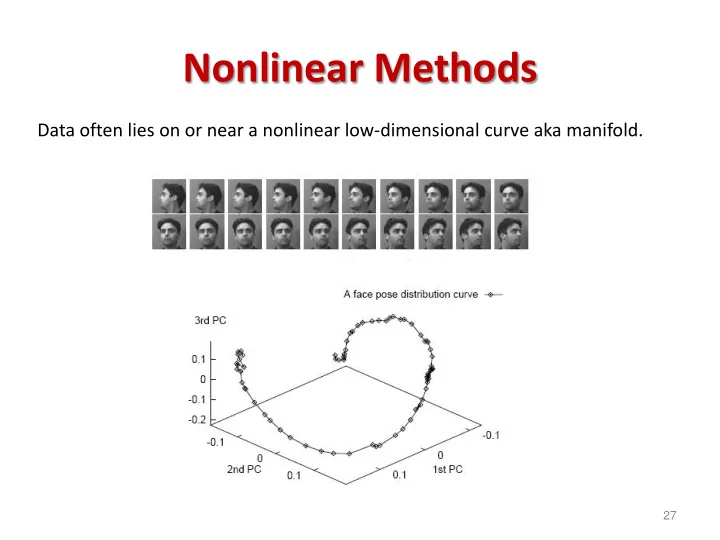
Data often lies on or near a nonlinear low-dimensional curve aka manifold.
27
Nonlinear Methods Data often lies on or near a nonlinear - - PowerPoint PPT Presentation
Nonlinear Methods Data often lies on or near a nonlinear low-dimensional curve aka manifold. 27 Laplacian Eigenmaps Linear methods Lower-dimensional linear projection that preserves distances between all points Laplacian Eigenmaps (key idea)
Data often lies on or near a nonlinear low-dimensional curve aka manifold.
27
Linear methods – Lower-dimensional linear projection that preserves distances between all points Laplacian Eigenmaps (key idea) – preserve local information only
Construct graph from data points (capture local information) Project points into a low-dim space using “eigenvectors of the graph”
Directed nearest neighbors (symmetric) kNN graph mutual kNN graph
Similarity Graphs: Model local neighborhood relations between data points G(V,E) V – Vertices (Data points) (1) E – Edge if ||xi – xj|| ≤ ε ε – neighborhood graph (2) E – Edge if k-NN, yields directed graph connect A with B if A → B OR A ← B (symmetric kNN graph) connect A with B if A → B AND A ← B (mutual kNN graph)
Similarity Graphs: Model local neighborhood relations between data points Choice of ε and k : Chosen so that neighborhood on graphs represent neighborhoods on the manifold (no “shortcuts” connect different arms of the swiss roll) Mostly ad-hoc
Similarity Graphs: Model local neighborhood relations between data points G(V,E,W) V – Vertices (Data points) E – Edges (nearest neighbors) W - Edge weights E.g. 1 if connected, 0 otherwise (Adjacency graph) Gaussian kernel similarity function (aka Heat kernel) s2 →∞ results in adjacency graph
L = D – W W – Weight matrix D – Degree matrix = diag(d1, …., dn) Note: If graph is connected, 1 is an eigenvector
.
L = D – W Solve generalized eigenvalue problem Order eigenvalues 0 = l1 ≤ l2 ≤ l3 ≤ … ≤ ln To embed data points in d-dim space, project data points onto eigenvectors associated with l2, l3, …, ld+1 ignore 1st eigenvector – same embedding for all points Original Representation Transformed representation data point projections xi → (f2(i), …, fd+1(i)) (D-dimensional vector) (d-dimensional vector)
Laplacian eigenvectors
(for large # data points)
possible after embedding
= LHS RHS = fT(D-W) f =
possible after embedding constraint removes arbitrary scaling factor in embedding Lagrangian:
Wrap constraint into the
N=number of nearest neighbors, t = the heat kernel parameter (Belkin & Niyogi’03)
Dimensional space.)
verbs prepositions
PCA Laplacian Eigenmaps Linear embedding Nonlinear embedding based on largest eigenvectors of based on smallest eigenvectors of D x D correlation matrix S = XXT n x n Laplacian matrix L = D – W between features between data points eigenvectors give latent features eigenvectors directly give
embedding of data points project them onto the latent features
xi → [f2(i), …, fd+1(i)]T
D x1 d x1 D x1 d x1
Score features (mutual information, prediction accuracy, domain knowledge) Regularization
more efficient representation than observed feature
Linear: Low-dimensional linear subspace projection PCA (Principal Component Analysis), MDS (Multi Dimensional Scaling), Factor Analysis, ICA (Independent Component Analysis) Nonlinear: Low-dimensional nonlinear projection that preserves local information along the manifold Laplacian Eigenmaps ISOMAP, Kernel PCA, LLE (Local Linear Embedding), Many, many more …
40