6.1 Dimensionality reduction Previously in the course, we have - PDF document

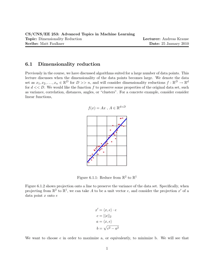
CS/CNS/EE 253: Advanced Topics in Machine Learning Topic: Dimensionality Reduction Lecturer: Andreas Krause Scribe: Matt Faulkner Date: 25 January 2010 6.1 Dimensionality reduction Previously in the course, we have discussed algorithms suited for a large number of data points. This lecture discusses when the dimensionality of the data points becomes large. We denote the data set as x 1 , x 2 , . . . , x n ∈ R D for D >> n , and will consider dimensionality reductions f : R D → R d for d << D . We would like the function f to preserve some properties of the original data set, such as variance, correlation, distances, angles, or “clusters”. For a concrete example, consider consider linear functions, f ( x ) = Ax , A ∈ R d × D Figure 6.1.1: Reduce from R 2 to R 1 Figure 6.1.2 shows projection onto a line to preserve the variance of the data set. Specifically, when projecting from R 2 to R 1 , we can take A to be a unit vector e , and consider the projection x ′ of a data point x onto e x ′ = � x, e � · e c = || x || 2 a = � x, e � � c 2 − a 2 b = We want to choose e in order to maximize a, or equivalently, to minimize b. We will see that 1

Figure 6.1.2: Choosing e to maximize the variance of the projection maximizes the a component over all data points; equivalently, choosing e to minimize reconstruction error minimizes b for all data points. “Maximize variance” ↔ “Minimize reconstruction error.” Principal component analysis (PCA) [3] is one such technique for projecting inputs onto a lower dimensional space so as to maximize variance. The desired orthogonal projection matrix A ∈ R d × D can be expressed as � � � � A ∗ = � � � � argmin x i − � x i , e j � · e j � � � � A =( e 1 ,...,e j ) ∈ R d × D i j � � 2 � � � � � � � � = argmax � x i , e j � · e j � � � � A =( e 1 ,...,e j ) ∈ R d × D i j � � 2 � � � x i , e j � 2 = j i Thus we see that this optimization has a closed-form solution. Now, assume d = 1. � x i , e 1 � 2 � max || e x ||≤ 1 i n || e x ||≤ 1 e T � x i · x T max i e 1 1 i i = 1 n x i · x T Noting that � i = n · Cov( X ) and letting C denote the covariance matrix, we get that the maximization can be expressed in terms of the Rayleigh quotient, e T 1 Ce 1 max e T 1 e 1 e 1 2

This is maximized by selecting e 1 as the eigenvector corresponding to the largest eigenvalue. For d − dimensional projection ( d > 1), if we let e 1 , . . . , e D denote the eigenvectors of the covariance matrix C corresponding to eigenvalues λ 1 ≥ · · · ≥ λ D , then the d − dimensional projection matrix is given by A ∗ = ( e 1 , . . . , e d ) 6.2 Preserving distances We would like to produce a faithful reduction, in that nearby inputs should be mapped to nearby outputs in lower dimensions. Motivated by this, we can formulate an optimization that seeks for each x i a ψ i ∈ R d s.t. || x i − x j || 2 − || ψ i − ψ j || 2 � � � min ψ i,j Intuitively, this minimizes the “stress” or the “distortion” of the dimension reduction. This opti- mization has a closed-form solution. Further, preserving distances turns out to be equivalent to preserving dot products: � ( � x i − x j � − � ψ i − ψ j � ) 2 min ψ i,j This is convenient because the reduction can be formulated for anything with a dot product, allowing the use of kernel tricks. This optimization, known as multidimensional scaling (MDS) [4] [2], also has a closed form solution. Define S i,j = || x i = x j || 2 to be the matrix of squared pairwise distances in the input space. We can then define the Gram matrix G i,j = � x i , x j � . This matrix can be derived from S as G = 1 2( I − uu T ) S ( I − uu T ) where u is the unit length vector 1 u = √ n (1 , . . . , 1) Here, the terms ( I = uu T ) have the effect of subtracting off the means of the data poitns, matk- The optimal solution ψ ∗ is computable from the eigenvectors of ing G a covariance matrix. the Gram matrix. Letting ( v i , . . . , v n ) be the eigenvectors of G with corresponding eigenvalues ( µ 1 , . . . , µ n ), the optimum ψ results from projecting each data point x i onto the d (scaled) eigen- vectors √ µ 1 v 1 , . . . , √ µ d v d . i,j = √ µ j v j · x i ψ ∗ For the optimal solution ψ ∗ it holds that ψ ∗ = A PCA x i , so PCA and MDS give equivalent results. However, PCA uses C = XX T ∈ R DxD , while DS uses G = X T X ∈ R nxn . These computational differences are summarized in Table 1. MDS also works whenever a distance metric exists between the data objects, so the objects are not required to be vectors. 3

6.3 Isomap: preserving distances along a manifold Suppose that the data set possesses a more complex structure, such as for the “Swiss Roll” in Fig. 6.3.3. Linear projections would do poorly, but it is clear that the data live in some lower- dimensional space. Figure 6.3.3: The Swiss Roll data set. A key insight is that within a small neighborhood of points, a linear method works well. We would like these local results to be consistent. One algorithm which formalizes this idea is Isomap [6]. Roughly, the algorithm performs three computations: 1. Construct a graph hby connecting k nearest neighbors, as in Fig. 6.3.4. 2. Define a metric d ( x i , x j ) = length of shortest path on graph from x i to x j . This is the “geodesic distance”. 3. Plug this distance metric into MDS. The result is that the distance between two points A and B on the roll respects the “path” through the manifold of data. 6.4 Maximal Variance unfolding Maximal variance unfolding (MVU) [7] is another dimensionality reduction technique that “pulls apart” the input data while trying to preserve distances and angles between nearby data points. Formally, it computes 4

Figure 6.3.4: Graph of four nearest neighbors on the Swiss Roll. Algorithm Primary computation Complexity C = XX T ∈ R DxD nD 2 PCA G = X T X ∈ R nxn n 2 D MDS n 2 log n + n 2 D ISOMAP geodesics and MDS n 6 MVU semidefinite programming Table 1: Computational efficiency of dimensionality reduction algorithms. � || ψ i || 2 max 2 X i || ψ i || 2 2 = || x i − x j || 2 subject to � ψ i = 0 , ∀ i, j i A closed-form solution for this problem does not exist, but it can be optimally solved using semidef- inite programming. 6.5 Computational Summary Table 1 summarizes the computational complexity of the dimensionality reduction algorithms con- sidered so far. Notably, the choice between PCA and MDS may depend on the relative size of the input n and its dimensionality D . 5

6.6 Random projections For comparison, what if A is picked at random? For linear dimension reduction only, consider choosing the entries of the matrix A as A i,j ∼ N (0 , 1) or � 1 +1 with prob 2 A i,j = 1 − 1 with prob 2 Somewhat surprisingly, this A can work well. Theorem 6.6.1 (Johnson & Lindenstrauss) Given n data points, for any ǫ > 0 and d = Θ( ǫ − 2 log n ) , with high probability (1 − ǫ ) || x i − x j || 2 ≤ || Ax i − Ax j || ≤ || x i − x j || (1 + ǫ ) 6.7 Further reading A few good surveys on dimensionality reduction exist, such as those by Saul [5], and Burges [1]. References [1] Christopher J. C. Burges. Geometric methods for feature extraction and dimensional reduction. In In L. Rokach and O. Maimon (Eds.), Data . Kluwer Academic Publishers, 2005. [2] TF Cox and MAA Cox. Multidimensional Scaling. Number 59 in Monographs on statistics and applied probability. Chapman & Hall. Pages , 30:31, 1994. [3] IT Jolliffe. Principal component analysis . Springer verlag, 2002. [4] J. Kruskal. Multidimensional scaling by optimizing goodness of fit to a nonmetric hypothesis. Psychometrika , 29(1):1–27, March 1964. [5] L.K. Saul, K.Q. Weinberger, J.H. Ham, F. Sha, and D.D. Lee. Spectral methods for dimension- ality reduction. Semisupervised Learning. MIT Press, Cambridge, MA , 2006. [6] J.B. Tenenbaum, V. Silva, and J.C. Langford. A global geometric framework for nonlinear dimensionality reduction. Science , 290(5500):2319, 2000. [7] K.Q. Weinberger and L.K. Saul. Unsupervised learning of image manifolds by semidefinite programming. International Journal of Computer Vision , 70(1):77–90, 2006. 6