Machine Learning 2 DS 4420 - Spring 2020 Dimensionality reduction 2 - PowerPoint PPT Presentation
Machine Learning 2 DS 4420 - Spring 2020 Dimensionality reduction 2 Byron C Wallace Today A bit of wrap up on PCA Then : Non-linear dimensionality reduction! (SNE/t-SNE) In Sum: Principal Component Analysis X = ( x 1 x
Machine Learning 2 DS 4420 - Spring 2020 Dimensionality reduction 2 Byron C Wallace
Today • A bit of wrap up on PCA • Then : Non-linear dimensionality reduction! (SNE/t-SNE)
In Sum: Principal Component Analysis X = ( x 1 · · · · · · x n ) ∈ R d ⇥ n Data Eigenvectors of Covariance λ 1 λ 2 Λ = ... λ d Idea : Take top- k eigenvectors to maximize variance
Why? Idea : Take top- k eigenvectors to maximize variance Last time, we saw that we can derive this by maximizing the variance in the compressed space
Why? Idea : Take top- k eigenvectors to maximize variance Last time, we saw that we can derive this by maximizing the variance in the compressed space Can also motivate by explicitly minimizing reconstruction error
Minimizing reconstruction error
Getting the eigenvalues, two ways • Direct eigenvalue decomposition of the covariance matrix N S = 1 n = 1 X N XX > x n x > N n =1
Getting the eigenvalues, two ways • Direct eigenvalue decomposition of the covariance matrix N S = 1 n = 1 X N XX > x n x > N n =1 • Singular Value Decomposition (SVD)
Singular Value Decomposition Idea : Decompose the d x n matrix X into 1. A n x n basis V (unitary matrix) 2. A d x n matrix Σ (diagonal projection) 3. A d x d basis U (unitary matrix) d X = U d ⇥ d Σ d ⇥ n V > n ⇥ n
2 1. Rotation n X V T ~ h ~ x i ~ x = v i , ~ e i i = 1 2. Scaling n X SV T ~ s i h ~ x i ~ x = v i , ~ e i i = 1 3. Rotation n X USV T ~ s i h ~ x i ~ x = v i , ~ u i i = 1
SVD for PCA V > = U X Σ , |{z} |{z} |{z} |{z} D ⇥ N D ⇥ D D ⇥ N N ⇥ N S = 1 N XX > = 1 Σ > U > = 1 N U Σ V > V N U ΣΣ > U > | {z } = I N
SVD for PCA V > = U X Σ , |{z} |{z} |{z} |{z} D ⇥ N D ⇥ D D ⇥ N N ⇥ N S = 1 N XX > = 1 Σ > U > = 1 N U Σ V > V N U ΣΣ > U > | {z } = I N It turns out the columns of U are the eigenvectors of XX T
Computing PCA Method 1: eigendecomposition n XX > U are eigenvectors of covariance matrix C = 1 Computing C already takes O ( nd 2 ) time (very expensive) Method 2: singular value decomposition (SVD) Find X = U d ⇥ d Σ d ⇥ n V > n ⇥ n where U > U = I d ⇥ d , V > V = I n ⇥ n , Σ is diagonal Computing top k singular vectors takes only O ( ndk )
Computing PCA Method 1: eigendecomposition n XX > U are eigenvectors of covariance matrix C = 1 Computing C already takes O ( nd 2 ) time (very expensive) Method 2: singular value decomposition (SVD) Find X = U d ⇥ d Σ d ⇥ n V > n ⇥ n where U > U = I d ⇥ d , V > V = I n ⇥ n , Σ is diagonal Computing top k singular vectors takes only O ( ndk ) Relationship between eigendecomposition and SVD: Left singular vectors are principal components ( C = U Σ 2 U > )
Eigen-faces [Turk & Pentland 1991] • d = number of pixels • Each x i 2 R d is a face image • x ji = intensity of the j -th pixel in image i
Eigen-faces [Turk & Pentland 1991] • d = number of pixels • Each x i 2 R d is a face image • x ji = intensity of the j -th pixel in image i X d × n U d × k Z k × n u ) ( z 1 . . . z n ) ) u ( ( . . .
Eigen-faces [Turk & Pentland 1991] • d = number of pixels • Each x i 2 R d is a face image • x ji = intensity of the j -th pixel in image i X d × n U d × k Z k × n u ) ( z 1 . . . z n ) ) u ( ( . . . Idea: z i more “meaningful” representation of i -th face than x i Can use z i for nearest-neighbor classification
Eigen-faces [Turk & Pentland 1991] • d = number of pixels • Each x i 2 R d is a face image • x ji = intensity of the j -th pixel in image i X d × n U d × k Z k × n u ) ( z 1 . . . z n ) ) u ( ( . . . Idea: z i more “meaningful” representation of i -th face than x i Can use z i for nearest-neighbor classification Much faster: O ( dk + nk ) time instead of O ( dn ) when n, d � k
Aside: How many components? • • Magnitude of eigenvalues indicate fraction of variance captured. • Eigenvalues on a face image dataset: 1353.2 1086.7 820.1 λ i 553.6 287.1 2 3 4 5 6 7 8 9 10 11 i • Eigenvalues typically drop o ff sharply, so don’t need that many. • Of course variance isn’t everything...
Wrapping up PCA • PCA is a linear model for dimensionality reduction which finds a mapping to a lower dimensional space that maximizes variance • We saw that this is equivalent to performing an eigendecomposition on the covariance matrix of X • Next time Auto-encoders and neural compression for non-linear projections
Wrapping up PCA • PCA is a linear model for dimensionality reduction which finds a mapping to a lower dimensional space that maximizes variance • We saw that this is equivalent to performing an eigendecomposition on the covariance matrix of X • Next time Auto-encoders and neural compression for non-linear projections
Non-linear dimensionality reduction
Limitations of Linearity PCA is e ff ective PCA is ine ff ective
Nonlinear PCA Broken solution Desired solution u 1 x 2 We want desired solution: S = { ( x 1 , x 2 ) : x 2 = u 2 1 }
Nonlinear PCA Broken solution Desired solution u 1 x 2 We want desired solution: S = { ( x 1 , x 2 ) : x 2 = u 2 1 } Idea: Use kernels 1 , x 2 ) > We can get this: S = { φ ( x ) = Uz } with φ ( x ) = ( x 2 { } Linear dimensionality reduction in φ ( x ) space ⇔ Nonlinear dimensionality reduction in x space
Kernel PCA
Alternatively: t-SNE !
Stochastic Neighbor Embeddings Borrowing from : Laurens van der Maaten (Delft -> Facebook AI)
Manifold learning Idea : Perform a non-linear dimensionality reduction in a manner that preserves proximity (but not distances)
Manifold learning
PCA on MNIST digits
t-SNE on MNIST Digits
Swiss roll Euclidean distance is not always a good notion of proximity
Non-linear projection Bad projection: relative position to neighbors changes
Non-linear projection Intuition: Want to preserve local neighborhood
Stochastic Neighbor Embedding Original space The map
SNE to t-SNE ( on board )
t-SNE: SNE with a t-Distribution Similarity in High Dimension exp ( − || x i − x j || 2 / 2 σ 2 ) p ij = k 6 = l exp ( − || x l − x k || 2 / 2 σ 2 ) P Similarity in Low Dimension (1 + || y i − y j || 2 ) � 1 q ij = k 6 = l (1 + || y k − y l || 2 ) � 1 P Gradient ∂ C ( p ij − q ij )(1 + || y i − y j || 2 ) � 1 ( y i − y j ) X = 4 ∂ y i j 6 = i
Algorithm 1 : Simple version of t-Distributed Stochastic Neighbor Embedding. Data : data set X = { x 1 , x 2 ,..., x n } , cost function parameters: perplexity Perp , optimization parameters: number of iterations T , learning rate η , momentum α ( t ) . Result : low-dimensional data representation Y ( T ) = { y 1 , y 2 ,..., y n } . begin compute pairwise affinities p j | i with perplexity Perp (using Equation 1) p j | i + p i | j set p ij = 2 n sample initial solution Y ( 0 ) = { y 1 , y 2 ,..., y n } from N ( 0 , 10 − 4 I ) for t=1 to T do compute low-dimensional affinities q ij (using Equation 4) compute gradient δ C δ Y (using Equation 5) set Y ( t ) = Y ( t − 1 ) + η δ C � Y ( t − 1 ) − Y ( t − 2 ) � δ Y + α ( t ) end end
Algorithm 1 : Simple version of t-Distributed Stochastic Neighbor Embedding. Data : data set X = { x 1 , x 2 ,..., x n } , cost function parameters: perplexity Perp , optimization parameters: number of iterations T , learning rate η , momentum α ( t ) . Result : low-dimensional data representation Y ( T ) = { y 1 , y 2 ,..., y n } . begin compute pairwise affinities p j | i with perplexity Perp (using Equation 1) p j | i + p i | j set p ij = 2 n sample initial solution Y ( 0 ) = { y 1 , y 2 ,..., y n } from N ( 0 , 10 − 4 I ) for t=1 to T do compute low-dimensional affinities q ij (using Equation 4) compute gradient δ C δ Y (using Equation 5) set Y ( t ) = Y ( t − 1 ) + η δ C � Y ( t − 1 ) − Y ( t − 2 ) � δ Y + α ( t ) end end
set Y ( t ) = Y ( t − 1 ) + η δ C � Y ( t − 1 ) − Y ( t − 2 ) � δ Y + α ( t )
set Y ( t ) = Y ( t − 1 ) + η δ C � Y ( t − 1 ) − Y ( t − 2 ) � δ Y + α ( t ) Regular gradient descent
“momentum” set Y ( t ) = Y ( t − 1 ) + η δ C � Y ( t − 1 ) − Y ( t − 2 ) � δ Y + α ( t )
Figure credit: Bisong, 2019
What’s magical about t ? Basically, the gradient has nice properties 18 Low − dimensional distance > 16 14 12 10 8 6 4 2 0 High − dimensional distance > (a) Gradient of SNE.
What’s magical about t ? Basically, the gradient has nice properties 18 Low − dimensional distance > 16 14 12 10 8 6 4 2 0 High − dimensional distance > (a) Gradient of SNE. Positive gradient —> “attraction” between points
What’s magical about t ? 18 1 Low − dimensional distance > Low − dimensional distance > 16 14 0.5 12 10 0 8 6 − 0.5 4 2 − 1 0 High − dimensional distance > High − dimensional distance > (a) Gradient of SNE. (c) Gradient of t-SNE. Positive gradient —> “attraction” between points
Recommend
More recommend
Explore More Topics
Stay informed with curated content and fresh updates.


