Modelling the spectral evolution of supernova (with the JEKYLL - - PowerPoint PPT Presentation

Modelling the spectral evolution of supernova (with the JEKYLL code).

Mattias Ergon (Stockholm University)

In collaboration with Claes Fransson, Anders Jerkstrand, Markus Kromer, Cecilia Kozma and Kristoffer Spricer

∂ni ∂ t +∇⋅(ni u)=∑ r j ,i nj−ni∑ ri, j 1 c ∂ I ∂ t +n⋅∇ I=η−χ I

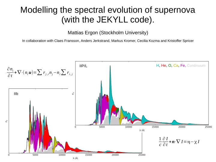
H, He, O, Ca, Fe, Continuum IIP/L IIb

The JEKYLL code

What: Realistic* simulations of the spectral evolution and lightcurves of SNe in the photospheric and nebular phase. How: Full NLTE-solution for the matter and the radiation field, following (and extending) the MC method outlined by Leon Lucy (2002, 2003, 2005). * Restrictions: Homologous expansion. Spherical symmetry. Steady-state for the matter (work in progress).

NLTE

NLTE: Non-LTE LTE: Local Thermodynamic Equilibrium In LTE all processes are in (near) equilibrium, and (given the density) the state is specified by a single parameter, the temperature.

Optically thick Optically thin Collisional processes dominate

NLTE Matter: LTE Radiation: NLTE LTE

NLTE

NLTE: Non-LTE LTE: Local Thermodynamic Equilibrium

NLTE

Yes No

In LTE all processes are in (near) equilibrium, and (given the density) the state is specified by a single parameter, the temperature.

Optically thick Optically thin Collisional processes dominate

NLTE Matter: LTE Radiation: NLTE LTE

NLTE

NLTE: Non-LTE LTE: Local Thermodynamic Equilibrium

NLTE

R a d i a t i v e t r a n s f e r e q u a t i

• n

NLTE rate equations Saha ionization and Boltzman excitation equation Diffusion approximation Yes No

In LTE all processes are in (near) equilibrium, and (given the density) the state is specified by a single parameter, the temperature.

Optically thick Optically thin Collisional processes dominate

NLTE Matter: LTE Radiation: NLTE LTE

NLTE

NLTE: Non-LTE LTE: Local Thermodynamic Equilibrium

NLTE

R a d i a t i v e t r a n s f e r e q u a t i

• n

NLTE rate equations

In the outer parts and at late times, SNe ejecta are neither optically thick, nor collisionally dominated, so a full NLTE solution is required.

Saha ionization and Boltzman excitation equation Diffusion approximation Yes No

In LTE all processes are in (near) equilibrium, and (given the density) the state is specified by a single parameter, the temperature.

Electron temperature Thermal energy equation Radiation field (MC) Radiative transfer Ion level populations NLTE rate equations Matter Lambda iteration Non-thermal electrons Spencer-Fano equation Time evolution

Method outline

MC radiative transfer

Following and extending the method by Lucy (2002, 2003, 2005).

MC radiative transfer

r i r

Ionization Recombination

... Following and extending the method by Lucy (2002, 2003, 2005). The MC packets carry energy. Radiation packets are propagated and interacts with the matter. When absorbed, packets are converted into excitation, ionization or thermal energy. When emitted, packets are converted into radiation energy.

MC radiative transfer

Rule number one: The MC packet energy is conserved. The MC packets carry energy. Radiation packets are propagated and interacts with the matter. When absorbed, packets are converted into excitation, ionization or thermal energy. When emitted, packets are converted into radiation energy. r i r

Ionization Recombination

... Following and extending the method by Lucy (2002, 2003, 2005).

Radioactive decays

γ γ

e

Compton scattering

Non-thermal electrons

e

Radioactive decays

γ γ

e

Ionization Heating Excitation Compton scattering Thermalization cascade

Non-thermal electrons

Non-thermal electrons

e

Radioactive decays

γ γ

e

Ionization Heating Excitation Compton scattering Thermalization cascade

Non-thermal electrons

Spencer-Fano (Boltzman) equation Non-thermal electron distribution Problem solved by Kozma & Fransson (1998), and their original FORTRAN routine has been integrated into JEKYLL.

Non-thermal electrons

Microscopic

Mixing

Hydrodynamical instabilities → Macroscopic mixing of the nuclear burning zones.

Macroscopic

Microscopic

Mixing

Hydrodynamical instabilities → Macroscopic mixing of the nuclear burning zones. Macroscopic vs Microscopic mixing Different composition and (possibly) density Different temperature, degree of ionizaton etc.

Macroscopic

Microscopic

Mixing

Hydrodynamical instabilities → Macroscopic mixing of the nuclear burning zones. To simulate macroscopic mixing, JEKYLL supports virtual cells (Jerkstrand et al. 2011). Virtual cells represents clumps of macroscopically mixed material, and are randomly selected while the photons traverse the otherwise spherically symmetric ejecta. Macroscopic vs Microscopic mixing Different composition and (possibly) density Different temperature, degree of ionizaton etc.

Macroscopic

Other similar codes

SUMO (Jerkstrand et al. 2011)

Geometry: 1-D NLTE: Full Non-thermal ionization/excitation: Yes Time-dependence: No Macroscopic mixing: Yes Phase: Nebular

ARTIS (Kromer et al. 2009)

Geometry: 3-D NLTE: Ionization Non-thermal ionization/excitation: No Time-dependence: Radiation field Macroscopic mixing: Yes Phase : Photospheric

CMFGEN (Hillier 1998)

Geometry: 1-D NLTE: Full Non-thermal ionization/excitation: Yes Time-dependence: Full Macroscopic mixing: No Phase: All

JEKYLL (Ergon et al. In prep.)

Geometry: 1-D NLTE: Full Non-thermal ionization/excitation: Yes Time-dependence: Radiation field Macroscopic mixing: Yes Phase: All

SEDONA (Kasen et al. 2006)

Geometry: 3-D NLTE: No Non-thermal ionization/excitation: No Time-dependence: Radiation field Macroscopic mixing: Yes Phase : Photospheric

+ Mazzali (2000,2001), Kerzendorf et al. (2014) and more.

Comparisons

JEKYLL and SUMO JEKYLL (circles) and ARTIS (crosses) CMFGEN

In progress. T.B.D.

Nebular spectra for Type IIb model 13G Early lightcurves for Type IIb model 12C

Comparisons

JEKYLL and CMFGEN

Constructed and evolved through the nebular phase with SUMO in Jerkstrand et al. (2015).

Type IIb models: Background

Evolved through the photospheric phase with JEKYLL in Ergon et al. (in prep). In the following I show results for model 12C, which showed a reasonable agreement with SN 2011dh in the nebular phase.

C/O He H 56Ni

MEj=1.7 M⊙ MNi=0.075M⊙ EK=6.8×10

50 erg

MIn=12M⊙

Type IIb models: Spectral evolution

Model 12C: Before 150 days H, He, O, Ca, Fe, Continuum

Comparison to SN 2011dh: Spectral evolution

Model 12C and SN 2011dh – Before 150 days

Comparison to SN 2011dh: Helium lines

Model 12C and SN 2011dh – Before 100 days Radioactive energy deposition in the helium envelope

Comparison to SN 2011dh: Lightcurves

Model 12C (circles) and SN 2011dh (crosses): Before 150 days

Effect of NLTE: Bolometric lightcurve

Model 12C : 3-100 days Model 12C: Before 100 days

Non-thermal ionization/excitation - Off Model 12C : 3-100 days Model 12C: Before 100 days

Effect of NLTE: Bolometric lightcurve

LTE Non-thermal ionization/excitation - Off Model 12C : 3-100 days Model: Before 100 days

Effect of NLTE: Bolometric lightcurve

Model 12C: Before 100 days

Model 12C : 3-100 days Model: Before 100 days

Effect of NLTE: Ionization

Non-thermal processes - On (circles) / Off (crosses) C/O core Inner He envelope Outer He envelope H envelope

Effect of NLTE: Spectral evolution

Non-thermal ionization/excitation - On/Off

Effect of NLTE: Broadband lightcurves

NLTE (circles) / LTE (crosses) Non-thermal processes - On (circles) / Off (crosses)

LTE + Opacity floor (HYDE) Model 12C : 3-100 days Model 12C: Before 100 days

Effect of NLTE: Bolometric lightcurve

LTE + Opacity floor (HYDE) Model 12C : 3-100 days Arnett (1982) + Popov (1991) Model 12C: Before 100 days

Effect of NLTE: Bolometric lightcurve

Effect of macroscopic mixing: Spectral evolution

Macroscopic mixing - On/Off

Effect of macroscopic mixing: Spectral evolution

Macroscopic mixing - On/Off

MH-Env=0.8 M⊙ MNi=0.1M⊙ EK=1×10

51 erg

MHe-Core=4.0M⊙

Type IIL SNe: A model with strong He lines

H, He, O, Ca, Fe, Continuum

MNi=0.1M⊙ EK=1×10

51 erg

MC/O-Core=2.9M⊙

Type Ic SNe: A model with strong Si lines

Si, He, O, Ca, Fe, Continuum Spectrum @ max Arnett (1982) + Popov (1991) Bolometric lightcurve