
SLIDE 1
May 30, 2005 Matlab Tutorial
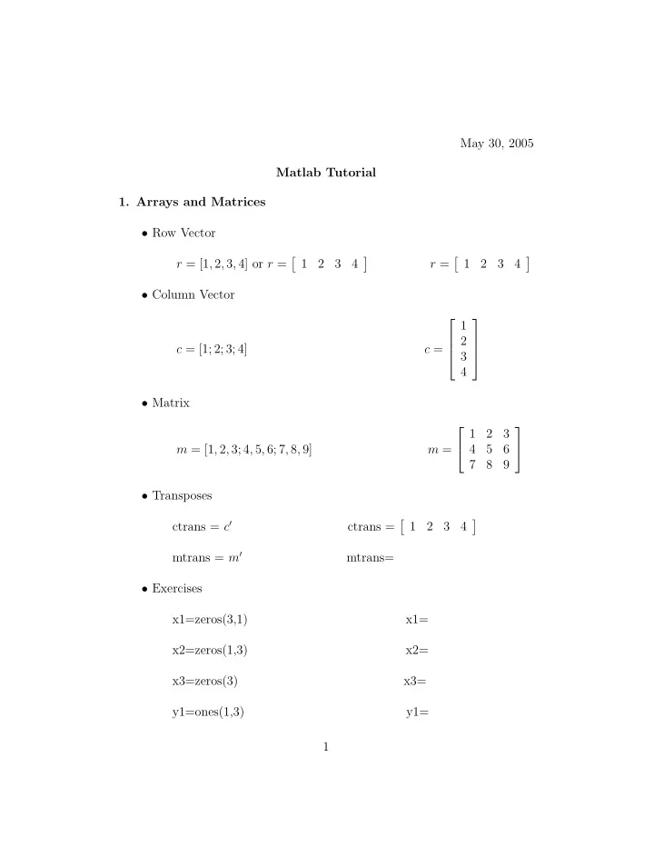
- 1. Arrays and Matrices
- Row Vector
r = [1, 2, 3, 4] or r =
- 1
2 3 4
- r =
- 1
2 3 4
- Column Vector
c = [1; 2; 3; 4] c = 1 2 3 4
- Matrix
m = [1, 2, 3; 4, 5, 6; 7, 8, 9] m = 1 2 3 4 5 6 7 8 9
- Transposes
ctrans = c′ ctrans =
- 1
2 3 4
- mtrans = m′
mtrans=
- Exercises