SLIDE 1 Engine workshop 5 Strassbourg 14. – 15.09.2006
Silke Köhler1, Felix Ziegler2
1GeoForschungsZentrum Potsdam (GFZ) 2Technical University of Berlin (TUB)
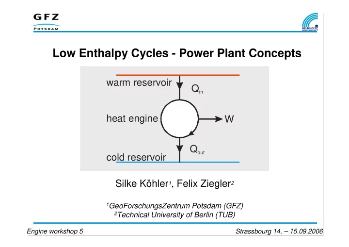
Low Enthalpy Cycles - Power Plant Concepts
warm reservoir cold reservoir Qout Qin W heat engine
SLIDE 2 Situation Heat source
Temperature 100°C – 200°C Mass flow rate 50 – 200 m³/h (~14 – 55 kg/s) Limited heat capacity ~ 5 to 50 MWth per well Sensible heat
Goal: Electricity generation Tools
Cycles and systems Design and optimisation Suitability of different cycles for particular applications
entropy temperature
heat source heat sink cyclic process
SLIDE 3
Optimisation of Ideal (Reversible) Cycles Internally and externally reversible
Carnot Cycle Lorentz Cycle Triangular Cycle
Internally reversible
Rankine Cycle - ideal cycle for steam power processes
Optimisation of the cycle locates the operating conditions for the optimal ideal cycle performance (Tamm et.al.)! Optimisation approach:
Locate constraints Locate free variables Define optimisation criterium objective function Find Max / Min by analytical or numerical solving of the function T, p
SLIDE 4
rejected heat qout: A A14B
area A 1234 Thermal efficiency η: area ratio
entropy temperature
1 2 3 4 A B
Carnot Cycle
∫
= Tds q
qin: A A23B qout: A A14B A A23B A 1234
∫
= − = Tds q q w
in
SLIDE 5 entropy temperature
heat source heat sink Carnot cycle
Optimisation of Carnot Cycle Constraints
Brine temperature, mass flow rate Heat sink temperature
Free variable
Upper process temperature Te
in r b
in in
q T Tds q q w q q , 1
,
∫
= − = − = η
Possible objective functions
Thermal efficiency η Net Work w Added heat qin / Cooling of the brine Tb,r
SLIDE 6 Optimisation of Carnot Cycle
entropy temperature
heat source heat sink Carnot cycle
entropy temperature
heat source heat sink
entropy temperature
heat source heat sink
entropy temperature
heat source heat sink
entropy temperature
heat source heat sink
entropy temperature
heat source heat sink Carnot cycle
η ↑ w ↓ Tb,r ↑ η ↓ w ↓ Tb,r ↓
SLIDE 7 entropy temperature
heat source heat sink Carnot cycle
Optimisation of Carnot Cycle Constraints
Brine temperature, mass flow rate Heat sink temperature
Free variable
Upper process temperature
Possible objective functions
Thermal efficiency η Net Work w Cooling of the brine Tb,r
b u
q T Tds q q w q q , 1
,
∫
= − = − = η
∫
= − = Tds q q w
u
SLIDE 8 Lorentz Cycle
entropy temperature entropy temperature
heat source heat sink
Constraints
Brine temperature, mass flow rate Heat sink temperature
Free variable
Upper process temperature Te
Possible objective functions
Thermal efficiency η Net Work w Added heat qin / Cooling of the brine Tb,r
SLIDE 9 Optimisation of Lorentz Cycle
entropy temperature
heat source heat sink
entropy temperature
heat source heat sink
entropy temperature
heat source heat sink
η ↑ w ↓ Tb,r ↑
entropy temperature
heat source heat sink
entropy temperature
heat source heat sink
entropy temperature
heat source heat sink
η ↓ w ↓ Tb,r ↓
SLIDE 10 Reversible Triangular Cycle
entropy temperature
heat source heat sink
Fits in heat source / heat sink characteristics No optimisation Availability? – not all state changes can be realized with available hard ware Ideal cycles help to analyse complex problems Real cycles suffer losses
SLIDE 11
Rankine Cycle (Organic Working Fluid)
2 isentropic compression 4 evaporator 5 isentropic expansion 1 constant pressure heat rejection condenser constant pressure heat addition preheater, desuper- heater, 1 2 4 5 temperature entropy 1 2 KP pl pu Te Tc 4 5 6 3
SLIDE 12
Actual Vapor Power Cycle (Organic Working Fluid)
temperature entropy 1 2 KP pl pu Te Tc 4 5 6 3 2 irreversibility in the pump 3 pressure drop 4 pressure drop 5 irreversibility in the turbine 6 pressure drop 1 pressure drop 1 2 3 4 5 6 real cycle ideal cycle
SLIDE 13
Irreversible Heat Transfer
temperature entropy Te Tc real cycle DTin DTout
SLIDE 14
ORC Layout
evaporator preheater feed pump condenser turbine generator heat sink production well injection well cooling water pump down hole pump 1 2 3 4 5
G
SLIDE 15 Heat Transfer Diagram ORC
Constraints
Brine: Tb,in, mass flow rate, specific heat capacity Cooling medium: TCW,in, TCW,out, specific heat capacity
Free variables
Working fluid Te ∆Tmin,in, ∆Tmin,out
Objective function
Generator capacity Heat transfer area (Ratio heat transfer area / generator capacity, ~ €/kW)
5 3 Tb,out 4 Tb,in Te b r i n e DTmin,out Tc 2 transferred heat Qout Qin temperature 1 TCW,out TCW,in cooling water DTmin,in 6
SLIDE 16
Kalina KCS 34 Layout
7 6 basic solution rich vapor feed pump absorber turbine generator production well injection well down hole pump cooling water pump separator heat sink
G
1 2 5 6’’ 11 pre- heater desorber 4 poor solution LT-recuperator 3 6’ 8 9 10 4 HT- recuperator
SLIDE 17 Heat Transfer Diagram Kalina
cooling water desorber brine temperature transferred heat 1 10 6 5 Qout Qin preheater TCW,in TCW,out Tb,in Tb,out absorber
DTmin,in
DTmin,out DTmin,in HT-preheater 11 3 4 6’ 8 Qre LT- preheater
SLIDE 18 Constraints
Brine: Tb,in, mass flow rate, specific heat capacity Cooling medium: TCW,in, TCW,out, specific heat capacity
Free variables
Composition basic solution Pressure desorption Pressure absorption
- Mass flow rate basic solution
- Objective function
Generator capacity Heat transfer area (Ratio heat transfer area / generator capacity, ~ €/kW)
Heat Transfer Diagram Kalina
des
Q &
re
Q &
cooling water desorber brine temperature transferred heat HT-preheater 1 11 10 2 3 4 6 5 6’ 8 Qout Qin Qre preheater LT- preheater TCW,in TCW,out Tb,in Tb,out absorber
DTmin,in
DTmin,out DTmin,in
SLIDE 19 25 50 75 100 125 100°C 125°C 150°C 175°C 200°C (R290) (RC318) (R600a) (R600) (i-C5) initial temperature brine, (working fluid) return temperature brine (°C) air cooling water cooling
ORC
Return Temperature Brine, ORC & Kalina Optimised for work output
50 75 100 125 100°C 125°C 150°C 175°C 200°C initial temperature brine return temperature brine (°C) air cooling water cooling
Kalina
SLIDE 20 0% 2% 4% 6% 8% 10% 100°C 125°C 150°C 175°C 200°C (R290) (RC318) (R600a) (R600) (i-C5) initial temperature brine, (working fluid)
air cooling water cooling
ORC
Overall Efficiency ORC & Kalina
( )
,
T T c m P P P P Q P
in b b brine CWpump FeedPump DHpump gen brine net sys
− − − − = = η & &
0% 2% 4% 6% 8% 10% 100°C 125°C 150°C 175°C 200°C initial temperature brine
air cooling water cooling
Kalina
Optimised for work output
SLIDE 21
Conclusions of Comparison Both systems are suitable for power production from low enthalpy reservoirs With given constraints from heat source and heat sink
ORC cool the brine more Kalina reach higher thermal efficiency High parasitic loads at ORC, especially for air cooling ORC are more sensible to changes ORC of heat sink
Suitability of the systems
Kalina KCS34 up to 150 °C brine or CHP ORC from 150 °C brine temperature
Improvements
Supercritical ORC may improve thermal efficiency Other Kalina systems may improve cooling of brine
SLIDE 22 Geothermal Heat and Power
brine temperature > temperature for heating purposes Not necessarily simultaneous production
Serial
power plant
T s
waste heat heating station brine out brine electrical energy
T QH
heat to district heating system
Additional constraints due to heating demand! Outlet temperature brine Mass flow rate brine Parallel
T QH
brine out brine power plant
T s
waste heat heating station electrical energy heat to district heating system
brine temperature ≈ temperature for heating Subsystems compete
SLIDE 23 Neustadt-Glewe Constraints
Brine temperature, mass flow rate Heat sink temperature Heating capacity in district heating system
Free variable
Portion of brine through plant / upper process temperature
Objective functions
Generator capacity ~ Pmech Cooling of the brine Tb,out Resource Utilization Factor RUE (overall exergetic efficiency) brine exergy products exergy RUE =
( ) ( )
( ) ( )
, ,
s s T h h m s s T h h m P P
in in brine HS HS HS HS tem heatingsys p t
− ⋅ − − ⋅ − ⋅ − − ⋅ + − = & &
brine 98°C 110 m³/h
power plant generator capacity 210 kWel
T s
heating station 6 MW geothermal
th
11 MW total
th
heat to district heating system net capacity to grid
Tb,out
SLIDE 24 Brine 35 kg/s, 98 °C District heating system (assumed) 50 kg/s, 70/55, 3.1 MWth Working medium power plant Perflourpentane, water cooling 15/20
50 100 150 200 30 50 70 90 upper process temperature (°C) T, P_mech T bout (°C) P mech (kW)
Results of Optimisation
0.2 0.4 0.6 0.8 1 1.2 30 50 70 90 upper process temperature (°C) portion of brine through plant RUE
( )
b in b brine in
T T c m const Q
, , −
⋅ = = & &
SLIDE 25
Summary
ORC & Kalina follow the same rules, but deal differently with the losses. Losses
Irreversible heat transfer Internal irreversibilities (non-isentropic state changes turbine and pump, pressure losses) Parasitic loads (cycle pump, down hole pump, cooling devices)
Constraints
Heat source and heat sink
Free Variables
Layout Working fluid (medium, composition) Upper process temperature
Power plant: optimised for work output CHP: optimised for RUE