Logistics Checkpoint 1 all graded Intro to Sampling Theory Grades - - PDF document

1 Intro to Sampling Theory

Logistics

 Checkpoint 1 all graded

 Grades / comments on mycourses

 Project Proposals due tonight

 Please place in mycourses dropbox

 Questions?

Plan for today

 Sampling Theory

Approaches to modeling in CG

 How does one describe reality?

 Empirical -- Use measured data  Fixed model  Procedural Modeling

 Physical simulation  Heuristic

Sampling Theory

 The world is continuous  Like it or not, CG is discrete.

 We work using a discrete array of pixels  We use discrete values for color  We use discrete arrays and subdivisions for

specifying textures and surfaces

 Process of going from continuous to

discrete is called sampling.

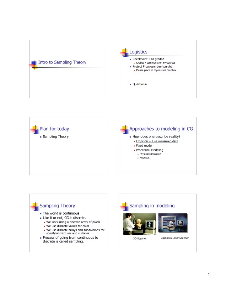
Sampling in modeling

3D Scanner Digibotics Laser Scanner

2

Sampling in modeling

Surface subdivision

Sampling in reflectance modeling

goniometer

Sampling in textures

www.sharkyextreme.com

Sampling in textures

Point sampled textures Filtered textures www.sharkyextreme.com

Sampling in image generation Sampling Theory

 Signal - function that conveys

information

 Audio signal (1D - function of time)  Image (2D - function of space)

 Continuous vs. Discrete

 Continuous - defined for all values in range  Discrete - defined for a set of discrete

points in range.

3

Sampling Theory

 Point Sampling

 start with continuous signal  calculate values of signal at discrete,

evenly spaced points (sampling)

 convert back to continuous signal for

display or output (reconstruction)

Sampling Theory

Foley/VanDam

Sampling Theory

 Sampling can be described as creating a

set of values representing a function evaluated at evenly spaced samples n i i f fn , , 2 , 1 , ) ( K =

• =

Δ = interval between samples = range / n.

Sampling Theory

 Sampling Rate = number of samples per unit  Example -- CD Audio

 sampling rate of 44,100 samples/sec  Δ = 1 sample every 2.26x10-5 seconds

• = 1

f

Issues:

 Important features of a scene may be

missed

 If view changes slightly or objects move

slightly, objects may move in and out of visibility.

 To fix, sample at a higher rate, but how

high does it need to be?

Sampling Theory

 Rich mathematical foundation for

sampling theory

 Hope to give an “intuitive” notion of

these mathematical concepts

4

Sampling Theory

 Spatial vs frequency domains

 Most well behaved functions can be

described as a sum of sin waves (possibly

• ffset) at various frequencies

 Frequency specturm - a function by the

contribution (and offset) at each frequency is describing the function in the frequency domain

 Higher frequencies equate to greater detail

Sampling Theory

Foley/VanDam

Sampling Theory

 Interactive wave builder  http://www.sunsite.ubc.ca/LivingMathe

matics/V001N01/UBCExamples/Fourier/f

• urier.html

Sampling Theory

 Annoying audio applet 1

 Fourier Synthesis -- Graphic Equalizer  http://www.phy.ntnu.edu.tw/ntnujava/vie

wtopic.php?t=33

Sampling Theory

 Nyquist Theorum

 A signal can be properly reconstructed if the signal

is sampled at a frequency (rate) that is greater than twice the highest frequency component of the signal.

 Said another way, if you have a signal with

highest frequency component of fh, you need at lease 2fh samples to represent this signal accurately.

Sampling Theory

 Example -- CD Audio

 sampling rate of 44,100 samples/sec  Δ = 1 sample every 2.26x10-5 seconds

 Using Nyquist Theorem

 CDs can accurately reproduce sounds with

frequencies as high as 22,050 Hz.

5

Sampling Theory

 Aliasing

 Failure to follow the Nyquist Theorum results in

aliasing.

 Aliasing is when high frequency components of a

signal appear as low frequency due to inadequate sampling.

 In CG:

 Jaggies (edges)  Textures  Missed objects

Sampling Theory

 Aliasing - example Foley/VanDam(628)

High frequencies masquerading as low frequencies

Sampling Theory

 Annoying Audio Applet 2

 Aliasing  http://ptolemy.eecs.berkeley.edu/eecs20/week13/

aliasing.html

Anti-Aliasing

 What to do in an aliasing situation

 Increase your sampling rate (supersampling)  Decrease the frequency range of your signal

(Filtering)

 How do we determine the contribution of

each frequency on our signal?

Fourier analysis

 Given f(x) we can generate a function

F(u) which indicates how much contribution each frequency u has on the function f.

 F(u) is the Fourier Transform  Fourier Transform has an inverse

Sampling Theory

 Fourier Transforms

Fourier Transform Inverse Fourier Transform f(x) F(u) f(x)

6

Sampling Theory

 The Fourier transform is defined as:

Note: the Fourier Transform is defined in the complex plane

• =

dt e t f u F

ut i 2

) ( ) (

Sampling Theory

 The Inverse Fourier transform is defined as:

• =

du e u F t f

ut i 2

) ( ) (

Signals in the frequency domain

 http://www.falstad.com/fourier/

Sampling Theory

 How do we calculate the Fourier

Transform?

 Use Mathematics  For discrete functions, use the Fast Fourier

Transform algorithm (FFT)

 Break…

Anti-Aliasing

 What to do in an aliasing situation

 Increase your sampling rate

(supersampling)

 Decrease the frequency range of your

signal (Filtering)

Supersampling

 Increase your sampling rate

 Examples

 Resolution in images  Number of subdivisions in modeling  Number of sample points  Number of rays per pixel.

 May not always have this luxury

7

Supersampling

Wikipedia

Anti-aliasing -- Filtering

 Can filter the transform to remove

• ffending high frequencies - partial

solution to anti-aliasing

 Removes high component frequencies from

a signal.

 Removing high frequencies results in

removing detail from the signal.

 Can be done in the frequency or spatial

domain

Getting rid of High Frequencies

 Filtering -- Frequency domain

 Place function into frequency domain F(u)  Simple multiplication with box filter S(u), aka

pulse function, band(width) limiting or low-pass filter.

 Suppress all frequency components above some specified cut-off

point k

• =

elsewhere , when , 1 ) ( k u k u S

Filtering – Frequency Domain

Foley/VanDam(631)

Original Spectrum Low-Pass Filter Spectrum with Filter Filtered Spectrum

Getting Rid of High Frequencies

 Filtering -- Spatial Domain

 Convolution (* operator) - equivalent to

multiplying two Fourier transforms

• =
• =
• d

x g f x g x f x h ) ( ) ( ) ( ) ( ) (

Taking a weighted average of the neighborhood around each point of f, weighted by g (the convolution or filter kernel) centered at that point.

Convultion sinc Function

 Convolving with a sinc function in the spatial

domain is the same as using a box filter in the frequency domain

Foley/VanDam (634)

FT→ ←FT-1

8

Filtering using Convolution

Foley/VanDam (633)

Original Spectrum Sinc Filter Spectrum with Filter value of filtered signal Filtered Spectrum

Convolution

 Joy of Convolution applet

http://www.jhu.edu/~signals/convolve/index. html

Sampling Theory

 Anti-aliasing -- Filtering

 Removes high component frequencies from

a signal.

 Removing high frequencies results in

removing detail from the signal.

 Can be done in the frequency or spatial

domain

Sampling Theory

 2D Sampling

 Images are examples of sampling in 2-

dimensions.

 2D Fourier Transforms provides strength of

signals at frequencies in the horizontal and vertical directions

Sampling Theory

 2D Aliasing

aliased image anti-aliased image

Foley/VanDam

Sampling Theory

 2D Fourier Transform

• +
• =

dxdy e y x f v u F

vy ux i ) ( 2

) , ( ) , (

9

Sampling Theory

   

Castleman

Sampling Theory

 Filtering - Convolution in 2D Castleman

Sampling Theory

 Filtering – Convolution with images Castleman

Sampling Theory

 Filtering – Convolution in frequency domain

Image 2D FFT Filter out high frequencies Filtered 2D FFT

Castleman

Other Anti-aliasing Methods

 Pre-filtering - filtering at object precision

before calculating pixel’s sample

 Post-filtering - supersampling (as we’ve seen)  Adaptive supersampling - sampling rate is

varied, applied only when needed (changes, edges, small items)

 Stochastic supersampling - places samples

at stocastically determined positions rather than regular grid

Anti-Aliasing

 Applet

http://www.nbb.cornell.edu/neurobio/land/Ol dStudentProjects/cs490- 96to97/anson/AntiAliasingApplet/index.html

10

Sampling Theory

 Summary

 Digital images are discrete with finite

resolution…the world is not.

 Spatial vs. Frequency domain  Nyquist Theorum  Convolution and Filtering  2D Convolution & Filtering  Questions?

Sampling Theory

 Further Reading

 Foley/VanDam – Chapter 14  Digital Image Processing by Kenneth

Castleman

 Glassner, Unit II (Book 1)

Remember

 Class Web Site:

 http://www.cs.rit.edu/~jmg/cgII

 Any questions?