Localization: Where am I? The map-building method we studied - - PDF document

SLIDE 1

1

Lecture 14: Localization

CS 344R/393R: Robotics Benjamin Kuipers

Thanks to Dieter Fox for some of his figures.

Localization: “Where am I?”

• The map-building method we studied

assumes that the robot knows its location.

– Precise (x,y,θ) coordinates in the same frame of reference as the occupancy grid map.

• This assumes that odometry is accurate,

which is often false.

• We will need to relocalize at each step.

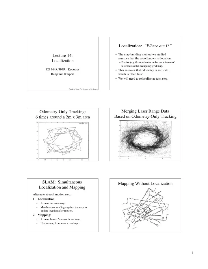
Odometry-Only Tracking: 6 times around a 2m x 3m area Merging Laser Range Data Based on Odometry-Only Tracking SLAM: Simultaneous Localization and Mapping

Alternate at each motion step:

• 1. Localization:
• Assume accurate map.
• Match sensor readings against the map to

update location after motion.

• 2. Mapping:
• Assume known location in the map.
• Update map from sensor readings.

Mapping Without Localization

SLIDE 2

2

Mapping With Localization Modeling Action and Sensing

• Action model: P(xt | xt-1, ut-1)
• Sensor model: P(zt | xt)
• What we want to know is Belief:

the posterior probability distribution of xt, given the past history of actions and sensor inputs. Xt-1 Xt Xt+1 Zt-1 Zt Zt+1 ut-1 ut

) , , , | ( ) (

1 2 1 t t t t

z u z u x P x Bel

• =

K

The Markov Assumption

• Given the present, the future is independent
• f the past.
• Given the state xt, the observation zt is

independent of the past.

Xt-1 Xt Xt+1 Zt-1 Zt Zt+1 ut-1 ut

P(zt | xt) = P(zt | xt,u1,z2 K,ut1)

Dynamic Bayesian Network

• The well-known DBN for local SLAM.

Law of Total Probability

(marginalizing)

• =

y

y x P x P ) , ( ) (

• =

y

y P y x P x P ) ( ) | ( ) (

P(y) =1

y

• Discrete

p(y) dy =1

• Continuous case
• =

dy y p y x p x p ) ( ) | ( ) (

• =

dy y x p x p ) , ( ) (

Bayes Law

• We can treat the denominator in Bayes Law

as a normalizing constant:

• We will apply it in the following form:

) ( ) | ( 1 ) ( ) ( ) | ( ) ( ) ( ) | ( ) (

1

x P x y P y P x P x y P y P x P x y P y x P

x

• =

= = =

• )

, , , | ( ) , , , , | (

1 2 1 1 2 1

• =

t t t t t

u z u x P u z u x z P K K

• )

, , , | ( ) (

1 2 1 t t t t

z u z u x P x Bel

• =

K

SLIDE 3

3

Bayes Filter

) , , , | ( ) , , , , | (

1 2 1 1 2 1

• =

t t t t t

u z u x P u z u x z P K K

• Bayes

) , , , | ( ) (

1 2 1 t t t t

z u z u x P x Bel

• =

K

Markov

) , , , | ( ) | (

1 2 1

• =

t t t t

u z u x P x z P K

• 1

1 1 1

) ( ) , | ( ) | (

• =

t t t t t t t

dx x Bel x u x P x z P

• Markov

1 1 2 1 1 1 1

) , , , | ( ) , | ( ) | (

• =

t t t t t t t t

dx u z u x P x u x P x z P K

• 1

1 2 1 1 1 1 2 1

) , , , | ( ) , , , , | ( ) | (

• =

t t t t t t t t

dx u z u x P x u z u x P x z P K K

• Total prob.

Markov Localization

• Bel(xt-1) and Bel(xt) are prior and posterior

probabilities of location x.

• P(xt | ut-1, xt-1) is the action model, giving the

probability distribution over result of ut-1 at xt-1.

• P(zt | xt) is the sensor model, giving the probability

distribution over sense images zt at xt.

• η is a normalization constant, ensuring that total

probability mass over xt is 1.

Bel(xt) = P(zt | xt) P(xt | ut1,xt1)

• Bel(xt1) dxt1

Markov Localization

• Evaluate Bel(xt) for every possible state xt.
• Prediction phase:

– Integrate over every possible state xt-1 to apply the probability that action ut-1 could reach xt from there.

• Correction phase:

– Weight each state xt with likelihood of observation zt.

Bel(xt) = P(xt | ut1,xt1)

• Bel(xt1) dxt1

Bel(xt) = P(zt | xt) Bel(xt)

Uniform prior probability Bel- (x0) Sensor information P(z0 | x0)

Bel(x0) = P(z0 | x0) Bel(x0)

Apply the action model P(x1 | u0, x0)

Bel(x1) = P(x1 | u0,x0)

• Bel(x0) dx0

SLIDE 4

4

Combine with observation P(z1 | x1)

Bel(x1) = P(z1 | x1) Bel(x1)

Action model again: P(x2 | u1, x1)

Bel(x2) = P(x2 | u1,x1)

• Bel(x1) dx1

Local and Global Localization

• Most localization is local:

– Incrementally correct belief in position after each action.

• Global localization is more dramatic.

– Where in the entire environment am I?

• The “kidnapped robot problem”

– Includes detecting that I am lost.

Initial belief Bel(x0) Intermediate Belief Bel(xt) Final Belief Bel(xt)

SLIDE 5

5

Global Localization Movie Future Attractions

• Sensor and action models
• Particle filtering

– elegant, simple algorithm – Monte Carlo simulation