lecture no 10
play

Lecture no: 10 Multicarrier systems History of multicarrier - PowerPoint PPT Presentation

RADIO SYSTEMS ETI 051 Contents Lecture no: 10 Multicarrier systems History of multicarrier Modulation/demodulation Equalization Multi-carrier Performance and Multiple antenna systems Different configuratuons


  1. RADIO SYSTEMS – ETI 051 Contents Lecture no: 10 • Multicarrier systems – History of multicarrier – Modulation/demodulation – Equalization Multi-carrier – Performance and • Multiple antenna systems – Different configuratuons Multiple antennas – Diversity gains – Datarates using MIMO (capacity) Ove Edfors, Department of Electrical and Information Technology Ove.Edfors@eit.lth.se 2010-05-06 Ove Edfors - ETI 051 1 2010-05-06 Ove Edfors - ETI 051 2 
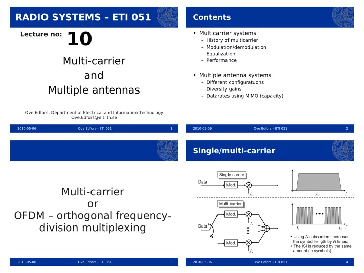
Single/multi-carrier Single carrier Single carrier Data Mod. Multi-carrier f C f C f or Multi-carrier Multi-carrier OFDM – orthogonal frequency- Mod. f 1 division multiplexing Data f f 1 f N • Using N cubcarriers increases the symbol length by N times. Mod. • The ISI is reduced by the same f N amount (in symbols). 2010-05-06 Ove Edfors - ETI 051 3 2010-05-06 Ove Edfors - ETI 051 4

  2. History and evolution [1] History and evolution [2] 1960’s : Subcarriers with overlapping spectra 1950’s : Few subcarriers, with non-overlapping spectra f f • Military systems, e.g. the Kineplex-modem Increased subchannel density and increased data rate. 2010-05-06 Ove Edfors - ETI 051 5 2010-05-06 Ove Edfors - ETI 051 6 History and evolution [3] History and evolution [4] 1980’s : Improved digital circuits increses interest 1970’s : Digital modulation of subcarriers No guard interval => Interference between both subcarriers and symbols Channel #n-1 #n #n+1 #n-1 #n #n+1 Analog modulation New digital modulation Analog modulation New digital modulation time time Mod. Guard interval => No interference between symbols Data Channel f 1 T Data F D/A #n-1 #n #n+1 #n-1 #n #n+1 D I time time f T X Cyclic prefix => No interference between neither subcarriers nor symbols Mod. Copy Copy Copy Copy f N { { { { #n-2 #n-1 #n #n+1 time 2010-05-06 Ove Edfors - ETI 051 7 2010-05-06 Ove Edfors - ETI 051 8

  3. Transmitters and receivers History and evolution [5] An N-subcarrier transmitter • 1990’s : Commercial applications appear s 0, k k – symbol x 0, k – Increased interest for OFDM in wireless applications s 1, k m – sample Parallel to serial x 1, k N-point IDFT – First applications in broadcasting (Audio/Video) n – subcarrier L – CP length s  t  – One of the candidates for UMTS (Beta proposal) h T CP T s p – sampling period X a m – Applied in wireless LANs 1 2 3 h T X – TX filter s N − 1, k x N − 1, k L = 3 N = 8 • 2000’s : One of the really hot technologies x n , k exp  j2  mn N  for 0 ≤ m ≤ N − 1 1 N − 1 – 54 Mbps and beyond WLANs (based on OFDM) hit the mass N-point IDFT: s m , k = 1 N ∑ market (IEEE802.11g/n) n = 0 2 – OFDM is the technology used when improving and moving Adding CP: s m , k = s N  m , k for − L ≤ m ≤− 1 beyond current 3G systems (LTE – long term evolution) s  t  = h TX  t  ∗  ∑ s m , k   t −  k  N  L   m  T samp   3 N − 1 k ∑ TX filtering: m =− L 2010-05-06 Ove Edfors - ETI 051 9 2010-05-06 Ove Edfors - ETI 051 10 Transmitters and receivers Transmitters and receivers ... through the channel ... N-subcarrier receiver Channel Noise n  t  h ch  t  r 0, k s  t  r  t  = s  t  ∗ h ch  t   n  t  q – symbol y 0, k r 1, k p – sample Serial to parallel y 1, k N-point DFT n – subcarrier t T samp r  t  } L – CP length T ch h R CP X T s p – sampling period a m 1 2 3 h R X – RX filter s  t  r  t  r N − 1, k y N − 1, k L = 3 N = 8 CP CP CP CP 1 z  t  = h RX  t  ∗ r  t   RX filtering: t t } } z  k T samp  LT samp T ch z k = Sampling: 2 As long as the CP is longer than the delay spread of the r p ,q = z q  N  L   p for 0 ≤ p ≤ N − 1 Removing CP: channel, LT s p > T c h , it will absorb the ISI. a m r p , q exp  − j2  np N  for 0 ≤ n ≤ N − 1 N − 1 3 y n , q = ∑ By removing the CP in the receiver, the transmission becomes N-point DFT: ISI free. p = 0 2010-05-06 Ove Edfors - ETI 051 11 2010-05-06 Ove Edfors - ETI 051 12

  4. Transmitters and receivers Transmitters and receivers Modulation spectrum [1] Modulation spectrum [2] The distance between each subcarrier The total modulation spectrum is 1 /  N T samp  Transmitted OFDM symbol decomposed Power spectrum of one subcarrier becomes which is the same a sum of the individual subcarrier into different subcarriers (ideal case, transmitted at f n Hz. as the 3 dB bandwidth of the individual spectra (assuming independent 4 subcarriers shown, no CP) subcarriers. Using all N subcarriers (8 data on them). 2   f − f n  N T samp  S n  f  ∝ sinc in this case) we get: S n  f n  1 2 S n  f n  t f N T samp f n f f 1 /  N T samp  N - Subcarriers B = N × 1 /  N T samp  = 1 / T samp B = 1 / T samp T samp - Sampling period sinc  x  = sin  x  x 2010-05-06 Ove Edfors - ETI 051 13 2010-05-06 Ove Edfors - ETI 051 14 Transmitters and receivers Transmitters and receivers Modulation spectrum [3] Simplified model Simplified model under ideal conditions Simplified model under ideal conditions (no fading and sufficient CP) (no fading and sufficient CP) 2048 subcarriers H 0, k n 0, k 64 subcarriers 0 0 ] ] x 0, k y 0, k B B Total filter in the signal path: d d -10 -10 [ [ y y t t h tot  t  = h TX  t  ∗ h ch  t  ∗ h RX  t  i i s s n -20 n -20 H N − 1, k n N − 1, k e e d d H tot  f  = H TX  f  × H ch  f  × H RX  f  l l a -30 a -30 r r t t c c e e x N − 1, k y N − 1, k p -40 p -40 s s r r e e w -50 w -50 o o P P Given that subcarrier n is -60 -60 -1.5 -1 -0.5 0 0.5 1 1.5 ν -1.5 -1 -0.5 0 0.5 1 1.5 ν transmitted at frequency f n Normalized frequency Normalized frequency the attenuations become: Normalized freq.: H n ,k = H tot  f n  = T samp f = f / B 2010-05-06 Ove Edfors - ETI 051 15 2010-05-06 Ove Edfors - ETI 051 16

  5. Transmitters and receivers Coded OFDM (CODFM) Focus on one subchannel Uncoded performance Before IDFT in TX After DFT in RX Before IDFT in TX After DFT in RX H n , k n n, k x n , k Subchannel k y n , k x n , k y n , k H n , k n n, k x n , k y n , k ∣ H n, k ∣ Amplitude scaling: PROBLEM: ∢ H n , k Rotation: • Only one fading tap per subchannel => NO DIVERSITY => POOR PERFORMANCE (16QAM) n n, k Noise: • The diversity is in there ... but additional techniques are needed to exploit it! SOLUTION: • Simple equalization of each subchannel: Back-rotate and scale • Spreading the information (data) across several subcarriers or OFDM symbols • This can be done using interleaving and coding => Coded OFDM (CODFM) 2010-05-06 Ove Edfors - ETI 051 17 2010-05-06 Ove Edfors - ETI 051 18 Coded OFDM (CODFM) Coded OFDM (CODFM) Channel correlation Coding and interleaving New blocks Frequency One OFDM symbol Channel attenuations (Corresponding ones at RX) Channel attenuation are correlated in the Parallel to serial time/frequency grid. N-point IDFT If we spread each bit of information over several h T CP Coding Interleaving X N subcarriers well separated points in the OFDM time/frequency grid, the same ”bit” is is received over several ”one tap” fading channels. Interleaving can be performed: Combining these in the - across subcarriers in The code spreads The interleaver reorders receiver, we obtain diversity. an OFDM symbol (small delay) the information the code symbols so that across several neighbouring code symbols - in time over several code symbols. are ”well” separated in OFDM symbols (longer delay) Time frequency and/or time during - or in a combination transmission. of the above. 2010-05-06 Ove Edfors - ETI 051 19 2010-05-06 Ove Edfors - ETI 051 20

  6. Coded OFDM (CODFM) Diversity The better the coding and interleaving scheme, the larger the obtained diversity order. Bit error rate (4QAM) 10 0 Multiple antenna systems Rayleigh fading 10 dB No diversity 10 -1 or = uncoded OFDM 10 x 10 -2 MIMO – multiple input/multiple output 10 dB Rayleigh fading 10 -3 K th order diversity (Coded OFDM) 10 -4 10 K x 10 -5 No fading 10 -6 0 2 4 6 8 10 12 14 16 18 20 E b /N 0 [dB] 2010-05-06 Ove Edfors - ETI 051 21 2010-05-06 Ove Edfors - ETI 051 22 System model [2] System model [3] An improvement : Antenna diversity A simple model : Superposition of received waves 1 [Movement -> fading] TX diversity (MISO): 2 1 h 1,2 ] [ x 2 ]  n 1 x 1 y 1 = [ h 1,1 h 1 RX diversity (SIMO): No diversity (SISO): 2 x [ y 2 ] = [ h 2,1 ] x 1  [ n 2 ] = + 1 y hx n y 1 h 1,1 n 1 TX RX 1 1 TX&RX diversity (MIMO): 2 2 Fading -> Poor performance [ y 2 ] = [ h 2,2 ][ x 2 ]  [ n 2 ] y 1 h 1,1 h 1,2 x 1 n 1 h 2,1 2010-05-06 Ove Edfors - ETI 051 23 2010-05-06 Ove Edfors - ETI 051 24

Download Presentation
Download Policy: The content available on the website is offered to you 'AS IS' for your personal information and use only. It cannot be commercialized, licensed, or distributed on other websites without prior consent from the author. To download a presentation, simply click this link. If you encounter any difficulties during the download process, it's possible that the publisher has removed the file from their server.

Recommend


More recommend