Lecture 7 LVCSR Training and Decoding (Part A) Michael Picheny, - - PowerPoint PPT Presentation

lecture 7
SMART_READER_LITE
LIVE PREVIEW

Lecture 7 LVCSR Training and Decoding (Part A) Michael Picheny, - - PowerPoint PPT Presentation

Lecture 7 LVCSR Training and Decoding (Part A) Michael Picheny, Bhuvana Ramabhadran, Stanley F . Chen, Markus Nussbaum-Thom Watson Group IBM T.J. Watson Research Center Yorktown Heights, New York, USA


slide-1
SLIDE 1

Lecture 7

LVCSR Training and Decoding (Part A) Michael Picheny, Bhuvana Ramabhadran, Stanley F . Chen, Markus Nussbaum-Thom

Watson Group IBM T.J. Watson Research Center Yorktown Heights, New York, USA {picheny,bhuvana,stanchen,nussbaum}@us.ibm.com

Mar 9, 2016

slide-2
SLIDE 2

Administrivia

Lab 2 Handed back this lecture or next. Lab 3 extension Due nine days from now (Friday, Mar. 18) at 6pm. Visit to IBM Watson Astor Place April 1, 11am. (About 1h?) Spring recess next week; no lecture.

2 / 96

slide-3
SLIDE 3

Feedback

Clear (9) Pace: fast (1) Muddiest: context models (3); diagonal GMM splitting (2); arcs v. state probs (1) Comments (2+ votes): Nice song (4) Hard to see chalk on blackboard (3) Lab 3 better than Lab 2 (2) Miss Michael on right (1); prefer Michael on left (1)

3 / 96

slide-4
SLIDE 4

The Big Picture

Weeks 1–4: Signal Processing, Small vocabulary ASR. Weeks 5–8: Large vocabulary ASR. Week 5: Language modeling (for large vocabularies). Week 6: Pronunciation modeling — acoustic modeling for large vocabularies. Week 7, 8: Training, decoding for large vocabularies. Weeks 9–13: Advanced topics.

4 / 96

slide-5
SLIDE 5

Outline

Part I: The LVCSR acoustic model. Part II: Acoustic model training for LVCSR. Part III: Decoding for LVCSR (inefficient). Part IV: Introduction to finite-state transducers. Part V: Search (Lecture 8). Making decoding for LVCSR efficient.

5 / 96

slide-6
SLIDE 6

Part I The LVCSR Acoustic Model

6 / 96

slide-7
SLIDE 7

What is LVCSR?

Demo from https://speech-to-text-demo.mybluemix.net/

7 / 96

slide-8
SLIDE 8

What is LVCSR?

Large vocabulary Continuous Speech Recognition. Phone-based modeling vs. word-based modeling. Continuous. No pauses between words.

8 / 96

slide-9
SLIDE 9

How do you evaluate such an LVCSR system?

Hello how can I help you today Hello ___ can EYE help you TO today

Ground Truth ASR Insertion Error Substitutio n Error Deletio n Error

9 / 96

slide-10
SLIDE 10

What do we have to begin training an LVCSR system?

100s of hours of recordings from many speakers Audio Recording 1 Audio Recording 2

Transcript 1 Transcript 2 Parallel database of audio and transcript

LVCSR

Lexicon or dictionary

10 / 96

slide-11
SLIDE 11

The Fundamental Equation of ASR

w∗ = arg max

ω

P(ω|x) (1) = arg max

ω

P(ω)P(x|ω) P(x) (2) = arg max

ω

P(ω)P(x|ω) (3) w∗ — best sequence of words (class) x — sequence of acoustic vectors P(x|ω) — acoustic model. P(ω) — language model.

11 / 96

slide-12
SLIDE 12

The Acoustic Model: Small Vocabulary

Pω(x) =

  • A

Pω(x, A) =

  • A

Pω(A) × Pω(x|A) (4) =≈ max

A

Pω(A) × Pω(x|A) (5) = max

A T

  • t=1

P(at)

T

  • t=1

P( xt|at) (6) log Pω(x) = max

A

T

  • t=1

log P(at) +

T

  • t=1

log P( xt|at)

  • (7)

P( xt|at) =

M

  • m=1

λat,m

D

  • dim d

N(xt,d; µat,m,d, σat,m,d) (8)

12 / 96

slide-13
SLIDE 13

The Acoustic Model: Large Vocabulary

Pω(x) =

  • A

Pω(x, A) =

  • A

Pω(A) × Pω(x|A) (9) =≈ max

A

Pω(A) × Pω(x|A) (10) = max

A T

  • t=1

P(at)

T

  • t=1

P( xt|at) (11) log Pω(x) = max

A

T

  • t=1

log P(at) +

T

  • t=1

log P( xt|at)

  • (12)

P( xt|at) =

M

  • m=1

λat,m

D

  • dim d

N(xt,d; µat,m,d, σat,m,d) (13)

13 / 96

slide-14
SLIDE 14

What Has Changed?

The HMM. Each alignment A describes a path through an HMM. Its parameterization. In P( xt|at), how many GMM’s to use? (Share between HMM’s?)

14 / 96

slide-15
SLIDE 15

Describing the Underlying HMM

Fundamental concept: how to map a word (or baseform) sequence to its HMM. In training, map reference transcript to its HMM. In decoding, glue together HMM’s for all allowable word sequences.

15 / 96

slide-16
SLIDE 16

The HMM: Small Vocabulary

TEN

. . . . . .

FOUR

One HMM per word. Glue together HMM for each word in word sequence.

16 / 96

slide-17
SLIDE 17

The HMM: Large Vocabulary

T EH N

. . . . . .

F AO R

One HMM per phone. Glue together HMM for each phone in phone sequence. Map word sequence to phone sequence using baseform dictionary.

The rain in Spain falls . . . DH AX | R EY N | IX N | S P EY N | F AA L Z | . . .

17 / 96

slide-18
SLIDE 18

An Example: Word to HMM

18 / 96

slide-19
SLIDE 19

An Example: Words to HMMs

19 / 96

slide-20
SLIDE 20

An Example: Word to HMM to GMMs

A set of arcs in a Markov model are tied to one another if they are constrained to have identical output distributions

E_b E_b E_m E_m E_e E_e E phone

20 / 96

slide-21
SLIDE 21

Now, in this example . . . The rain in Spain falls . . . DH AX | R EY N | IX N | S P EY N | F AA L Z | . . .

38

N Is phone 2 positions to the left a vowel no yes Is phone 1 position to the left a long vowel {P EY N}, {R, EY, N}, { | IX N} {P EY N}, {R, EY, N} …. yes no {| IX N} Is phone 1 position to the left a boundary phone yes {| IX N} no Is phone 2 positions to the left a plosive yes {P EY N} {R, EY, N} no

21 / 96

slide-22
SLIDE 22

I Still Don’t See What’s Changed

HMM topology typically doesn’t change. HMM parameterization changes.

22 / 96

slide-23
SLIDE 23

Parameterization

Small vocabulary. One GMM per state (three states per phone). No sharing between phones in different words. Large vocabulary, context-independent (CI). One GMM per state. Tying between phones in different words. Large vocabulary, context-dependent (CD). Many GMM’s per state; GMM to use depends on phonetic context. Tying between phones in different words.

23 / 96

slide-24
SLIDE 24

Context-Dependent Parameterization

Each phone HMM state has its own decision tree. Decision tree asks questions about phonetic context. (Why?) One GMM per leaf in the tree. (Up to 200+ leaves/tree.) How will tree for first state of a phone tend to differ . . . From tree for last state of a phone? Terminology. triphone model — ±1 phones of context. quinphone model — ±2 phones of context.

24 / 96

slide-25
SLIDE 25

Example of Tying

Examples of “0” will affect models for “3” and “4” Useful in large vocabulary systems (why?)

25 / 96

slide-26
SLIDE 26

A Real-Life Tree

In practice: These trees are built on one-third of a phone, i.e., the three states of the HMM for a phone correspond to the beginning, middle and end of a phone. Context-independent versions Context-dependent versions

26 / 96

slide-27
SLIDE 27

Another Sample Tree

27 / 96

slide-28
SLIDE 28

Pop Quiz

System description: 1000 words in lexicon; average word length = 5 phones. There are 50 phones; each phone HMM has three states. Each decision tree contains 100 leaves on average. How many GMM’s are there in: A small vocabulary system (word models)? A CI large vocabulary system? A CD large vocabulary system?

28 / 96

slide-29
SLIDE 29

Context-Dependent Phone Models

Typical model sizes: GMM’s/ type HMM state GMM’s Gaussians word per word 1 10–500 100–10k CI phone per phone 1 ∼150 1k–3k CD phone per phone 1–200 1k–10k 10k–300k 39-dimensional feature vectors ⇒ ∼80 parameters/Gaussian. Big models can have tens of millions of parameters.

29 / 96

slide-30
SLIDE 30

Any Questions?

T EH N

. . . . . .

F AO R

Given a word sequence, you should understand how to . . . Layout the corresponding HMM topology. Determine which GMM to use at each state, for CI and CD models.

30 / 96

slide-31
SLIDE 31

What About Transition Probabilities?

This slide only included for completeness. Small vocabulary. One set of transition probabilities per state. No sharing between phones in different words. Large vocabulary. One set of transition probabilities per state. Sharing between phones in different words. What about context-dependent transition modeling?

31 / 96

slide-32
SLIDE 32

Recap

Main difference between small vocabulary and large vocabulary: Allocation of GMM’s. Sharing GMM’s between words: needs less GMM’s. Modeling context-dependence: needs more GMM’s. Hybrid allocation is possible. Training and decoding for LVCSR. In theory, any reason why small vocabulary techniques won’t work? In practice, yikes!

32 / 96

slide-33
SLIDE 33

Points to Ponder

Why deterministic mapping?

DID YOU ⇒ D IH D JH UW

The area of pronunciation modeling. Why decision trees? Unsupervised clustering.

33 / 96

slide-34
SLIDE 34

Part II Acoustic Model Training for LVCSR

34 / 96

slide-35
SLIDE 35

Small Vocabulary Training — Lab 2

Phase 1: Collect underpants. Initialize all Gaussian means to 0, variances to 1. Phase 2: Iterate over training data. For each word, train associated word HMM . . . On all samples of that word in the training data . . . Using the Forward-Backward algorithm. Phase 3: Profit!

35 / 96

slide-36
SLIDE 36

Large Vocabulary Training

What’s changed going to LVCSR? Same HMM topology; just more Gaussians and GMM’s. Can we just use the same training algorithm as before?

36 / 96

slide-37
SLIDE 37

Where Are We?

1

The Local Minima Problem

2

Training GMM’s

3

Building Phonetic Decision Trees

4

Details

5

The Final Recipe

37 / 96

slide-38
SLIDE 38

Flat or Random Start

Why does this work for small models? We believe there’s a huge global minimum . . . In the “middle” of the parameter search space. With a neutral starting point, we’re apt to fall into it. (Who knows if this is actually true.) Why doesn’t this work for large models?

38 / 96

slide-39
SLIDE 39

Training a Mixture of Two 2-D Gaussians

Flat start? Initialize mean of each Gaussian to 0, variance to 1.

  • 4
  • 2

2 4

  • 10
  • 5

5 10

39 / 96

slide-40
SLIDE 40

Training a Mixture of Two 2-D Gaussians

Random seeding? Picked 8 random starting points ⇒ 3 different optima.

  • 4
  • 2

2 4

  • 10
  • 5

5 10

40 / 96

slide-41
SLIDE 41

Training Hidden Models

(MLE) training of models with hidden variables has local minima. What are the hidden variables in ASR? i.e., what variables are in our model . . . That are not observed.

41 / 96

slide-42
SLIDE 42

How To Spot Hidden Variables

Pω(x) =

  • A

Pω(x, A) =

  • APω(A) × Pω(x|A)

(14) =≈ max

A

Pω(A) × Pω(x|A) (15) = max

A T

  • t=1

P(at)

T

  • t=1

P( xt|at) (16) log Pω(x) = max

A

T

  • t=1

log P(at) +

T

  • t=1

log P( xt|at)

  • (17)

P( xt|at) =

  • M

m=1λat,m D

  • dim d

N(xt,d; µat,m,d, σat,m,d) (18)

42 / 96

slide-43
SLIDE 43

Gradient Descent and Local Minima

EM training does hill-climbing/gradient descent. Finds “nearest” optimum to where you started.

likelihood parameter values

43 / 96

slide-44
SLIDE 44

What To Do?

Insight: If we know the “correct” hidden values for a model: e.g., which arc and which Gaussian for each frame . . . Training is easy! (No local minima.) Remember Viterbi training given fixed alignment in Lab 2. Is there a way to guess the correct hidden values for a large model?

44 / 96

slide-45
SLIDE 45

Bootstrapping Alignments

Recall that all of our acoustic models, from simple to complex: Generally use the same HMM topology! (All that differs is how we assign GMM’s to each arc.) Given an alignment (from arc/phone states to frames) for simple model . . . It is straightforward to compute analogous alignment for complex model!

45 / 96

slide-46
SLIDE 46

Bootstrapping Big Models From Small

Recipe: Start with model simple enough that flat start works. Iteratively build more and more complex models . . . By using last model to seed hidden values for next. Need to come up with sequence of successively more complex models . . . With related hidden structure.

46 / 96

slide-47
SLIDE 47

How To Seed Next Model From Last

Directly via hidden values, e.g., alignment. e.g., single-pass retraining. Can be used between very different models. Via parameters. Seed parameters in complex model so that . . . Initially, will yield same/similar alignment as in simple model. e.g., moving from CI to CD GMM’s.

47 / 96

slide-48
SLIDE 48

Bootstrapping Big Models From Small

Recurring motif in acoustic model training. The reason why state-of-the-art systems . . . Require many, many training passes, as you will see. Recipes handed down through the generations. Discovered via sweat and tears. Art, not science. But no one believes these find global optima . . . Even for small problems.

48 / 96

slide-49
SLIDE 49

Overview of Training Process

Build CI single Gaussian model from flat start. Use CI single Gaussian model to seed CI GMM model. Build phonetic decision tree (using CI GMM model to help). Use CI GMM model to seed CD GMM model.

49 / 96

slide-50
SLIDE 50

Where Are We?

1

The Local Minima Problem

2

Training GMM’s

3

Building Phonetic Decision Trees

4

Details

5

The Final Recipe

50 / 96

slide-51
SLIDE 51

Case Study: Training a GMM

Recursive mixture splitting. A sequence of successively more complex models. Perturb means in opposite directions; same variance; Train. (Discard Gaussians with insufficient counts.) k-means clustering. Seed means in one shot.

51 / 96

slide-52
SLIDE 52

Mixture Splitting Example

Split each Gaussian in two (±0.2 × σ)

  • 4
  • 2

2 4

  • 10
  • 5

5 10

52 / 96

slide-53
SLIDE 53

Applying Mixture Splitting in ASR

Recipe: Start with model with 1-component GMM’s (à la Lab 2). Split Gaussians in each output distribution simultaneously. Do many iterations of FB. Repeat. Real-life numbers: Five splits spread within 30 iterations of FB.

53 / 96

slide-54
SLIDE 54

Another Way: Automatic Clustering

Use unsupervised clustering algorithm to find clusters (k-Means Clustering) Given clusters . . . Use cluster centers to seed Gaussian means. FB training. (Discard Gaussians with insufficient counts.)

54 / 96

slide-55
SLIDE 55

k-Means Clustering

Select desired number of clusters k. Choose k data points randomly. Use these as initial cluster centers. “Assign” each data point to nearest cluster center. Recompute each cluster center as . . . Mean of data points “assigned” to it. Repeat until convergence.

55 / 96

slide-56
SLIDE 56

k-Means Example

Pick random cluster centers; assign points to nearest center.

  • 4
  • 2

2 4

  • 10
  • 5

5 10

56 / 96

slide-57
SLIDE 57

k-Means Example

Use centers as means of Gaussians; train, yep.

  • 4
  • 2

2 4

  • 10
  • 5

5 10

57 / 96

slide-58
SLIDE 58

The Final Mixtures, Splitting vs. k-Means

  • 4
  • 2

2 4

  • 10
  • 5

5 10

  • 4
  • 2

2 4

  • 10
  • 5

5 10

58 / 96

slide-59
SLIDE 59

Technical Aside: k-Means Clustering

When using Euclidean distance . . . k-means clustering is equivalent to . . . Seeding Gaussian means with the k initial centers. Doing Viterbi EM update, keeping variances constant.

59 / 96

slide-60
SLIDE 60

Applying k-Means Clustering in ASR

To train each GMM, use k-means clustering . . . On what data? Which frames? Huh? How to decide which frames align to each GMM? This issue is evaded for mixture splitting. Can we avoid it here?

60 / 96

slide-61
SLIDE 61

Forced Alignment

Viterbi algorithm. Finds most likely alignment of HMM to data.

P1(x) P1(x) P2(x) P2(x) P3(x) P3(x) P4(x) P4(x) P5(x) P5(x) P6(x) P6(x)

frame 1 2 3 4 5 6 7 8 9 10 11 12 arc P1 P1 P1 P2 P3 P4 P4 P5 P5 P5 P5 P6 P6

Need existing model to create alignment. (Which?)

61 / 96

slide-62
SLIDE 62

Recap

You can use single Gaussian models to seed GMM models. Mixture splitting: use c-component GMM to seed 2c-component GMM. k-means: use single Gaussian model to find alignment. Both of these techniques work about the same. Nowadays, we primarily use mixture splitting.

62 / 96

slide-63
SLIDE 63

Where Are We?

1

The Local Minima Problem

2

Training GMM’s

3

Building Phonetic Decision Trees

4

Details

5

The Final Recipe

63 / 96

slide-64
SLIDE 64

What Do We Need?

For each tree/phone state . . . List of frames/feature vectors associated with that tree. (This is the data we are optimizing the likelihood of.) For each frame, the phonetic context. A list of candidate questions about the phonetic context. Ask about phonetic concepts; e.g., vowel or consonant? Expressed as list of phones in set. Allow same questions to be asked about each phone position. Handed down through the generations.

64 / 96

slide-65
SLIDE 65

Training Data for Decision Trees

Forced alignment/Viterbi decoding! Where do we get the model to align with? Use CI phone model or other pre-existing model.

DH1 DH2 AH1 AH2 D1 D2 AO1 AO2 G1 G2

frame 1 2 3 4 5 6 7 8 9 · · · arc DH1 DH2 AH1 AH2 D1 D1 D2 D2 D2 AO1 · · ·

65 / 96

slide-66
SLIDE 66

Building the Tree

A set of events {( xi, pL, pR)} (possibly subsampled). Given current tree: Choose question of the form . . . “Does the phone in position j belong to the set q?” . . . That optimizes

i P(

xi|leaf(pL, pR)) . . . Where we model each leaf using a single Gaussian. Can efficiently build whole level of tree in single pass. See Lecture 6 slides and readings for the gory details.

66 / 96

slide-67
SLIDE 67

Seeding the Context-Dependent GMM’s

Context-independent GMM’s: one GMM per phone state. Context-dependent GMM’s: l GMM’s per phone state. How to seed context-dependent GMM’s? e.g., so that initial alignment matches CI alignment?

67 / 96

slide-68
SLIDE 68

Where Are We?

1

The Local Minima Problem

2

Training GMM’s

3

Building Phonetic Decision Trees

4

Details

5

The Final Recipe

68 / 96

slide-69
SLIDE 69

Where Are We?

4

Details Maximum Likelihood Training? Viterbi vs. Non-Viterbi Training Graph Building

69 / 96

slide-70
SLIDE 70

The Original Story, Small Vocabulary

One HMM for each word; flat start. Collect all examples of each word. Run FB on those examples to do maximum likelihood training of that HMM.

70 / 96

slide-71
SLIDE 71

The New Story

One HMM for each word sequence!? But tie parameters across HMM’s! Do complex multi-phase training. Are we still doing anything resembling maximum likelihood training?

71 / 96

slide-72
SLIDE 72

Maximum Likelihood Training?

Regular training iterations (FB, Viterbi EM). Increase (Viterbi) likelihood of data. Seeding last model from next model. Mixture splitting. CI ⇒ CD models. (Decision-tree building.)

72 / 96

slide-73
SLIDE 73

Maximum Likelihood Training?

Just as LM’s need to be smoothed or regularized. So do acoustic models. Prevent extreme likelihood values (e.g., 0 or ∞). ML training maximizes training data likelihood. We actually want to optimize test data likelihood. Let’s call the difference the overfitting penalty. The overfitting penalty tends to increase as . . . The number of parameters increase and/or . . . Parameter magnitudes increase.

73 / 96

slide-74
SLIDE 74

Regularization/Capacity Control

Limit size of model. Will training likelihood continue to increase as model grows? Limit components per GMM. Limit number of leaves in decision tree, i.e., number of GMM’s. Variance flooring. Don’t let variances go to 0 ⇒ infinite likelihood.

74 / 96

slide-75
SLIDE 75

Where Are We?

4

Details Maximum Likelihood Training? Viterbi vs. Non-Viterbi Training Graph Building

75 / 96

slide-76
SLIDE 76

Two Types of Updates

“Full” EM. Compute true posterior of each hidden configuration. Viterbi EM. Use Viterbi algorithm to find most likely hidden configuration. Assign posterior of 1 to this configuration. Both are valid updates; instances of generalized EM.

76 / 96

slide-77
SLIDE 77

Examples

Training GMM’s. Mixture splitting vs. k-means clustering. Training HMM’s. Forward-backward vs. Viterbi EM (Lab 2). Everywhere you do a forced alignment. Refining the reference transcript. What is non-Viterbi version of decision-tree building?

77 / 96

slide-78
SLIDE 78

When To Use One or the Other?

Which version is more expensive computationally? Optimization: need not realign every iteration. Which version finds better minima? If posteriors are very sharp, they do almost the same thing. Remember example posteriors in Lab 2? Rule of thumb: When you’re first training a “new” model, use full EM. Once you’re “locked in” to an optimum, Viterbi is fine.

78 / 96

slide-79
SLIDE 79

Where Are We?

4

Details Maximum Likelihood Training? Viterbi vs. Non-Viterbi Training Graph Building

79 / 96

slide-80
SLIDE 80

Building HMM’s For Training

When doing Forward-Backward on an utterance . . . We need the HMM corresponding to the reference transcript. Can we use the same techniques as for small vocabularies?

80 / 96

slide-81
SLIDE 81

Word Models

Reference transcript

THE DOG

Replace each word with its HMM

THE1 THE2 THE3 THE4 DOG1 DOG2 DOG3 DOG4 DOG5 DOG6

81 / 96

slide-82
SLIDE 82

Context-Independent Phone Models

Reference transcript

THE DOG

Pronunciation dictionary. Maps each word to a sequence of phonemes.

DH AH D AO G

Replace each phone with its HMM

DH1 DH2 AH1 AH2 D1 D2 AO1 AO2 G1 G2

82 / 96

slide-83
SLIDE 83

Context-Dependent Phone Models

THE DOG DH AH D AO G

DH1 DH2 AH1 AH2 D1 D2 AO1 AO2 G1 G2 DH1,3 DH2,7 AH1,2 AH2,4 D1,3 D2,9 AO1,1 AO2,1 G1,2 G2,7

83 / 96

slide-84
SLIDE 84

The Pronunciation Dictionary

Need pronunciation of every word in training data. Including pronunciation variants

THE(01)

DH AH

THE(02)

DH IY Listen to data? Use automatic spelling-to-sound models? Why not consider multiple baseforms/word for word models?

84 / 96

slide-85
SLIDE 85

But Wait, It’s More Complicated Than That!

Reference transcripts are created by humans . . . Who, by their nature, are human (i.e., fallible) Typical transcripts don’t contain everything an ASR system wants. Where silence occurred; noises like coughs, door slams, etc. Pronunciation information, e.g., was THE pronounced as DH UH or DH IY?

85 / 96

slide-86
SLIDE 86

Pronunciation Variants, Silence, and Stuff

How can we produce a more “complete” reference transcript? Viterbi decoding! Build HMM accepting all word (HMM) sequences consistent with reference transcript. Compute best path/word HMM sequence. Where does this initial acoustic model come from?

~SIL(01) THE(01) THE(02) ~SIL(01) DOG(01) DOG(02) DOG(03) ~SIL(01) ~SIL(01) THE(01) DOG(02) ~SIL(01)

86 / 96

slide-87
SLIDE 87

Another Way

Just use the whole expanded graph during training.

~SIL(01) THE(01) THE(02) ~SIL(01) DOG(01) DOG(02) DOG(03) ~SIL(01)

The problem: how to do context-dependent phone expansion? Use same techniques as in building graphs for decoding.

87 / 96

slide-88
SLIDE 88

Where Are We?

1

The Local Minima Problem

2

Training GMM’s

3

Building Phonetic Decision Trees

4

Details

5

The Final Recipe

88 / 96

slide-89
SLIDE 89

Prerequisites

Audio data with reference transcripts. What two other things?

89 / 96

slide-90
SLIDE 90

The Training Recipe

Find/make baseforms for all words in reference transcripts. Train single Gaussian models (flat start; many iters of FB). Do mixture splitting, say. Split each Gaussian in two; do many iterations of FB. Repeat until desired number of Gaussians per mixture. (Use initial system to refine reference transcripts.) Select pronunciation variants, where silence occurs. Do more FB training given refined transcripts. Build phonetic decision tree. Use CI model to align training data. Seed CD model from CI; train using FB or Viterbi EM. Possibly doing more mixture splitting.

90 / 96

slide-91
SLIDE 91

How Long Does Training Take?

It’s a secret. We think in terms of real-time factor. How many hours does it take to process one hour of speech?

91 / 96

slide-92
SLIDE 92

Whew, That Was Pretty Complicated!

Adaptation (VTLN, fMLLR, mMLLR) Discriminative training (LDA, MMI, MPE, fMPE) Model combination (cross adaptation, ROVER) Iteration. Repeat steps using better model for seeding. Alignment is only as good as model that created it.

92 / 96

slide-93
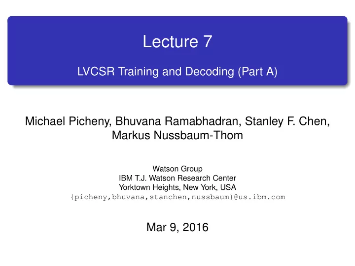
SLIDE 93

Things Can Get Pretty Hairy

ML-SAT-L ML-AD-L

ROVER

Consensus

rescoring 100-best rescoring 100-best 4-gram rescoring 4-gram rescoring 4-gram rescoring 4-gram rescoring 4-gram rescoring

Consensus Consensus Consensus Consensus Consensus

rescoring 100-best 4-gram rescoring 4-gram rescoring 4-gram rescoring 4-gram rescoring

Consensus Consensus Consensus

36.3%

MFCC ML-SAT-L VTLN ML-AD-L ML-SAT ML-AD MMI-SAT MMI-AD ML-SAT ML-AD MFCC-SI PLP VTLN MMI-SAT MMI-AD Consensus

4-gram 100-best rescoring rescoring 38.4% Eval’01 WER 35.6% 31.6% 30.3% 30.1% 30.5% 31.0% 32.1% 29.9% 31.1% 30.2% 28.8% 28.7% 31.4% 29.2% 27.8% 29.2% 29.5% 30.1% 29.8% 30.9% 31.9% 34.3% 42.6% 45.9% Eval’98 WER (SWB only) 34.0% 41.6% 39.3% 38.5% 37.7% 38.7% 38.1% 36.7% 38.7% 30.8% 37.9% 38.1% 37.1% 36.9% 35.9% 35.2% 35.7% 36.5% 38.1% 37.2% 35.5% 37.7%

93 / 96

slide-94
SLIDE 94

Recap: Acoustic Model Training for LVCSR

Take-home messages. Hidden model training is fraught with local minima. Seeding more complex models with simpler models helps avoid terrible local minima. People have developed many recipes/heuristics to try to improve the minimum you end up in. Training is insanely complicated for state-of-the-art research models. The good news . . . I just saved a bunch on money on my car insurance by switching to GEICO.

94 / 96

slide-95
SLIDE 95

Outline

Part I: The LVCSR acoustic model. Part II: Acoustic model training for LVCSR. Part III: Decoding for LVCSR (inefficient). Part IV: Introduction to finite-state transducers. Part V: Search (Lecture 8). Making decoding for LVCSR efficient.

95 / 96

slide-96
SLIDE 96

Course Feedback

1

Was this lecture mostly clear or unclear? What was the muddiest topic?

2

Other feedback (pace, content, atmosphere)?

96 / 96