Lecture 12 The remaining samples x 1 ,,x S is an approximation of - - PowerPoint PPT Presentation

▶

Oct 09, 2022 442 likes •506 views

METROPOLIS LOREM HASTINGS (MH) I P S U M Royal Institute of Technology We want to compute p*(x) (typically p(x|D)) STAT. METH. IN How? Implicitly construct Markov Chain M CS COLLAPSED with stationary distribution p*(x) GIBBS

SLIDE 1

LOREM

I P S U M

STAT. METH. IN

CS – COLLAPSED GIBBS SAMPLER

Lecture 12

Royal Institute of Technology

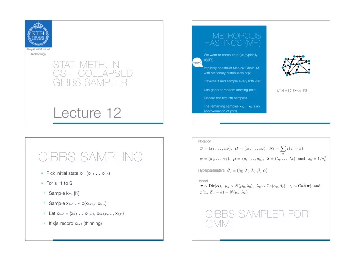
METROPOLIS HASTINGS (MH)

We want to compute p*(x) (typically p(x|D)) Implicitly construct Markov Chain M with stationary distribution p*(x) Traverse it and sample every k:th visit Use good or random starting point Discard the first l:th samples The remaining samples x1,…,xS is an approximation of p*(x) p*(x) ≈ [ ∑i I(x=xi) ]/S How?

GIBBS SAMPLING

★ Pick initial state x1=(x1,1,…,x1,K) ★ For s=1 to S

Sample k~u [K]
Sample xs+1,k ~ p(xs+1,k| xs,-k)
Let xs+1 = (xs,1,…,x1,k-1, xs+1,k,…, xs,K)
If k|s record xs+1 (thinning)

GIBBS SAMPLER FOR GMM

Notation Hyperparameters Model

D = (x1, . . . , xN), H = (z1, . . . , zN), Nk =

I(zi = k) π = (π1, . . . , πk), µ = (µi, . . . , µk), λ = (λi, . . . , λk), and λk = 1/σ2

θ0 = (µ0, λ0, λ0, β0, α) π ∼ Dir(α), µk ∼ N(µ0, λ0), λk ∼ Ga(α0, β0), zi ∼ Cat(π), and p(xn|Zn = k) = N(µk, λk)

SLIDE 2

A STATE

(H, π, µ, λ)

LIKELIHOOD FOR GMM

Hyperparameters Model Likelihood

θ0 = (µ0, λ0, λ0, β0, α) π ∼ Dir(α), µk ∼ N(µ0, λ0), λk ∼ Ga(α0, β0), zi ∼ Cat(π), and p(xn|Zn = k) = N(µk, λk) p(D, H, π, µ, λ) =p(D, H|π, µ, λ)p(π)p(µ, λ) =

[πkN(xn|µk, λk)]I(zn=k)Dir(π|α)

N(µk|µ0, λ0)Ga(λk|α0, β0)

COLLAPSING

Integrating out some components of the state is called collapsing It always improves convergence

10 10 1 10 2 10 3 −600 −550 −500 −450 −400 −350

Iteration log p(x | π, θ)

Standard Gibbs Sampler Rao−Blackwellized Sampler 10 10 1 10 2 10 3 −600 −550 −500 −450 −400 −350

Iteration log p(x | π, θ)

Standard Gibbs Sampler Rao−Blackwellized Sampler

COLLAPSING

Integrating out some components of the posterior is called collapsing It always improves convergence

10 10 1 10 2 10 3 −600 −550 −500 −450 −400 −350

Iteration log p(x | π, θ)

Standard Gibbs Sampler Rao−Blackwellized Sampler 10 10 1 10 2 10 3 −600 −550 −500 −450 −400 −350

Iteration log p(x | π, θ)

Standard Gibbs Sampler Rao−Blackwellized Sampler

SLIDE 3

COLLAPSED GIBBS SAMPLER FOR GMM

Integrate out π, μ, and λ from p(D,H,μ,λ,π,ϴ0) ϴ0 is all the hyperparameters Only full conditionals on zn remain Same joint as before except from conjugate prior on μk and λk

NEW FULL CONDITIONAL

“easy” with a conjugate prior on μk and λk but varies as we vary H

FULL CONDITIONAL

So,

α =

αk

where

π ∼ Dir(α), µk ∼ N(µ0, λ0), λk ∼ Ga(α0, β0), zi ∼ Cat(π), and p(xn|Zn = k) = N(µk, λk)

Recall, I.e., marginal

THE COLLAPSED ALGORITHM

SLIDE 4

CONVERGENC E COLLAPSED VS STANDARD

Blue is standard
Red is collapsed
x iterations
y loglikelihood

10 10 1 10 2 10 3 −600 −550 −500 −450 −400 −350

Iteration log p(x | π, θ)

Standard Gibbs Sampler Rao−Blackwellized Sampler 10 10 1 10 2 10 3 −600 −550 −500 −450 −400 −350

Iteration log p(x | π, θ)

Standard Gibbs Sampler Rao−Blackwellized Sampler

THE END

SLIDE 5 FIGURE 3. Comparison of the convergence time of PosetSMC and MCMC. We generated coalescent trees of different sizes and data sets

f 1000 nucleotides. We computed the L1 distance of the minimum Bayes risk reconstruction to the true generating tree as a function of the

running time (in units of the number of peeling recursions, on a log scale). The missing MCMC data points are due to MrBayes stalling on these executions.