Stochastic Simulation Idea: probabilities samples Get probabilities - - PowerPoint PPT Presentation

Stochastic Simulation

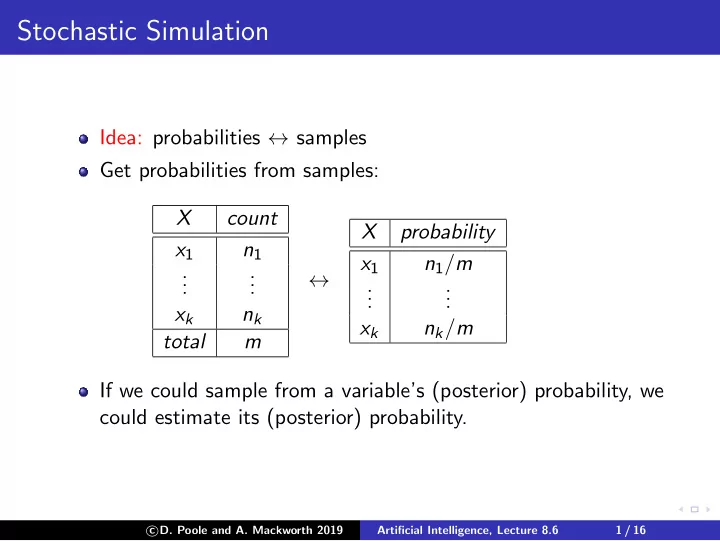
Idea: probabilities ↔ samples Get probabilities from samples: X count x1 n1 . . . . . . xk nk total m ↔ X probability x1 n1/m . . . . . . xk nk/m If we could sample from a variable’s (posterior) probability, we could estimate its (posterior) probability.

c

• D. Poole and A. Mackworth 2019

Artificial Intelligence, Lecture 8.6 1 / 16

Generating samples from a distribution

For a variable X with a discrete domain or a (one-dimensional) real domain: Totally order the values of the domain of X. Generate the cumulative probability distribution: f (x) = P(X ≤ x). Select a value y uniformly in the range [0, 1]. Select the x such that f (x) = y.

c

• D. Poole and A. Mackworth 2019

Artificial Intelligence, Lecture 8.6 2 / 16

Cumulative Distribution

v1 v2 v3 v4 v1 v2 v3 v4 P(X) f(X) 1 1

c

• D. Poole and A. Mackworth 2019

Artificial Intelligence, Lecture 8.6 3 / 16

Hoeffding’s inequality

Theorem (Hoeffding): Suppose p is the true probability, and s is the sample average from n independent samples; then P(|s − p| > ǫ) ≤ 2e−2nǫ2. Guarantees a probably approximately correct estimate of probability.

c

• D. Poole and A. Mackworth 2019

Artificial Intelligence, Lecture 8.6 4 / 16

Hoeffding’s inequality

Theorem (Hoeffding): Suppose p is the true probability, and s is the sample average from n independent samples; then P(|s − p| > ǫ) ≤ 2e−2nǫ2. Guarantees a probably approximately correct estimate of probability. If you are willing to have an error greater than ǫ in δ of the cases, solve 2e−2nǫ2 < δ for n, which gives

c

• D. Poole and A. Mackworth 2019

Artificial Intelligence, Lecture 8.6 4 / 16

Hoeffding’s inequality

Theorem (Hoeffding): Suppose p is the true probability, and s is the sample average from n independent samples; then P(|s − p| > ǫ) ≤ 2e−2nǫ2. Guarantees a probably approximately correct estimate of probability. If you are willing to have an error greater than ǫ in δ of the cases, solve 2e−2nǫ2 < δ for n, which gives n > − ln δ

2

2ǫ2 .

c

• D. Poole and A. Mackworth 2019

Artificial Intelligence, Lecture 8.6 4 / 16

Hoeffding’s inequality

Theorem (Hoeffding): Suppose p is the true probability, and s is the sample average from n independent samples; then P(|s − p| > ǫ) ≤ 2e−2nǫ2. Guarantees a probably approximately correct estimate of probability. If you are willing to have an error greater than ǫ in δ of the cases, solve 2e−2nǫ2 < δ for n, which gives n > − ln δ

2

2ǫ2 . ǫ δ n 0.1 0.05 185 0.01 0.05 18,445 0.1 0.01 265

c

• D. Poole and A. Mackworth 2019

Artificial Intelligence, Lecture 8.6 4 / 16

Forward sampling in a belief network

Sample the variables one at a time; sample parents of X before sampling X. Given values for the parents of X, sample from the probability

• f X given its parents.

c

• D. Poole and A. Mackworth 2019

Artificial Intelligence, Lecture 8.6 5 / 16

Rejection Sampling

To estimate a posterior probability given evidence Y1 = v1 ∧ . . . ∧ Yj = vj: Reject any sample that assigns Yi to a value other than vi. The non-rejected samples are distributed according to the posterior probability: P(α | evidence) ≈

• sample|

=α 1

• sample 1

where we consider only samples consistent with evidence.

c

• D. Poole and A. Mackworth 2019

Artificial Intelligence, Lecture 8.6 6 / 16

Rejection Sampling Example: P(ta | sm, re)

Ta Fi Sm Al Le Re

Observe Sm = true, Re = true Ta Fi Al Sm Le Re s1 false true false true false false

c

• D. Poole and A. Mackworth 2019

Artificial Intelligence, Lecture 8.6 7 / 16

Rejection Sampling Example: P(ta | sm, re)

Ta Fi Sm Al Le Re

Observe Sm = true, Re = true Ta Fi Al Sm Le Re s1 false true false true false false ✘ s2 false true true true true true

c

• D. Poole and A. Mackworth 2019

Artificial Intelligence, Lecture 8.6 7 / 16

Rejection Sampling Example: P(ta | sm, re)

Ta Fi Sm Al Le Re

Observe Sm = true, Re = true Ta Fi Al Sm Le Re s1 false true false true false false ✘ s2 false true true true true true ✔ s3 true false true false

c

• D. Poole and A. Mackworth 2019

Artificial Intelligence, Lecture 8.6 7 / 16

Rejection Sampling Example: P(ta | sm, re)

Ta Fi Sm Al Le Re

Observe Sm = true, Re = true Ta Fi Al Sm Le Re s1 false true false true false false ✘ s2 false true true true true true ✔ s3 true false true false — — ✘ s4 true true true true true true

c

• D. Poole and A. Mackworth 2019

Artificial Intelligence, Lecture 8.6 7 / 16

Rejection Sampling Example: P(ta | sm, re)

Ta Fi Sm Al Le Re

Observe Sm = true, Re = true Ta Fi Al Sm Le Re s1 false true false true false false ✘ s2 false true true true true true ✔ s3 true false true false — — ✘ s4 true true true true true true ✔ . . . s1000 false false false false

c

• D. Poole and A. Mackworth 2019

Artificial Intelligence, Lecture 8.6 7 / 16

Rejection Sampling Example: P(ta | sm, re)

Ta Fi Sm Al Le Re

Observe Sm = true, Re = true Ta Fi Al Sm Le Re s1 false true false true false false ✘ s2 false true true true true true ✔ s3 true false true false — — ✘ s4 true true true true true true ✔ . . . s1000 false false false false — — ✘ P(sm) = 0.02 P(re | sm) = 0.32 How many samples are rejected? How many samples are used?

c

• D. Poole and A. Mackworth 2019

Artificial Intelligence, Lecture 8.6 7 / 16

Importance Sampling

Samples have weights: a real number associated with each sample that takes the evidence into account. Probability of a proposition is weighted average of samples: P(α | evidence) ≈

• sample|

=α weight(sample)

• sample weight(sample)

Mix exact inference with sampling: don’t sample all of the variables, but weight each sample according to P(evidence | sample).

c

• D. Poole and A. Mackworth 2019

Artificial Intelligence, Lecture 8.6 8 / 16

Importance Sampling (Likelihood Weighting)

procedure likelihood weighting(Bn, e, Q, n): ans[1 : k] := 0 where k is size of dom(Q) repeat n times: weight := 1 for each variable Xi in order: if Xi = oi is observed weight := weight × P(Xi = oi | parents(Xi)) else assign Xi a random sample of P(Xi | parents(Xi)) if Q has value v: ans[v] := ans[v] + weight return ans/

v ans[v]

c

• D. Poole and A. Mackworth 2019

Artificial Intelligence, Lecture 8.6 9 / 16

Importance Sampling Example: P(ta | sm, re)

Ta Fi Sm Al Le Re

Ta Fi Al Le Weight s1 true false true false s2 false true false false s3 false true true true s4 true true true true . . . s1000 false false true true P(sm | fi) = 0.9 P(sm | ¬fi) = 0.01 P(re | le) = 0.75 P(re | ¬le) = 0.01

c

• D. Poole and A. Mackworth 2019

Artificial Intelligence, Lecture 8.6 10 / 16

Importance Sampling Example: P(ta | sm, re)

Ta Fi Sm Al Le Re

Ta Fi Al Le Weight s1 true false true false 0.01 × 0.01 s2 false true false false 0.9 × 0.01 s3 false true true true 0.9 × 0.75 s4 true true true true 0.9 × 0.75 . . . s1000 false false true true 0.01 × 0.75 P(sm | fi) = 0.9 P(sm | ¬fi) = 0.01 P(re | le) = 0.75 P(re | ¬le) = 0.01

c

• D. Poole and A. Mackworth 2019

Artificial Intelligence, Lecture 8.6 10 / 16

Importance Sampling Example: P(le | sm, ta, ¬re)

Ta Fi Sm Al Le Re

P(ta) = 0.02 P(fi) = 0.01 P(al | fi ∧ ta) = 0.5 P(al | fi ∧ ¬ta) = 0.99 P(al | ¬fi ∧ ta) = 0.85 P(al | ¬fi ∧ ¬ta) = 0.0001 P(sm | fi) = 0.9 P(sm | ¬fi) = 0.01 P(le | al) = 0.88 P(le | ¬al) = 0.001 P(re | le) = 0.75 P(re | ¬le) = 0.01

c

• D. Poole and A. Mackworth 2019

Artificial Intelligence, Lecture 8.6 11 / 16

Computing Expectations & Proposal Distributions

Expected value of f with respect to distribution P: EP(f ) =

• w

f (w) ∗ P(w)

c

• D. Poole and A. Mackworth 2019

Artificial Intelligence, Lecture 8.6 12 / 16

Computing Expectations & Proposal Distributions

Expected value of f with respect to distribution P: EP(f ) =

• w

f (w) ∗ P(w) ≈ 1 n

• s

f (s) s is sampled with probability P. There are n samples.

c

• D. Poole and A. Mackworth 2019

Artificial Intelligence, Lecture 8.6 12 / 16

Computing Expectations & Proposal Distributions

Expected value of f with respect to distribution P: EP(f ) =

• w

f (w) ∗ P(w) ≈ 1 n

• s

f (s) s is sampled with probability P. There are n samples. EP(f ) =

• w

f (w) ∗ P(w)/Q(w) ∗ Q(w)

c

• D. Poole and A. Mackworth 2019

Artificial Intelligence, Lecture 8.6 12 / 16

Computing Expectations & Proposal Distributions

Expected value of f with respect to distribution P: EP(f ) =

• w

f (w) ∗ P(w) ≈ 1 n

• s

f (s) s is sampled with probability P. There are n samples. EP(f ) =

• w

f (w) ∗ P(w)/Q(w) ∗ Q(w) ≈ 1 n

• s

f (s) ∗ P(s)/Q(s) s is selected according the distribution Q. The distribution Q is called a proposal distribution. P(c) > 0 then Q(c) > 0.

c

• D. Poole and A. Mackworth 2019

Artificial Intelligence, Lecture 8.6 12 / 16

Particle Filtering

Importance sampling can be seen as: for each particle: for each variable: sample / absorb evidence / update query where particle is one of the samples.

c

• D. Poole and A. Mackworth 2019

Artificial Intelligence, Lecture 8.6 13 / 16

Particle Filtering

Importance sampling can be seen as: for each particle: for each variable: sample / absorb evidence / update query where particle is one of the samples. Instead we could do: for each variable: for each particle: sample / absorb evidence / update query Why?

c

• D. Poole and A. Mackworth 2019

Artificial Intelligence, Lecture 8.6 13 / 16

Particle Filtering

Importance sampling can be seen as: for each particle: for each variable: sample / absorb evidence / update query where particle is one of the samples. Instead we could do: for each variable: for each particle: sample / absorb evidence / update query Why? We can have a new operation of resampling It works with infinitely many variables (e.g., HMM)

c

• D. Poole and A. Mackworth 2019

Artificial Intelligence, Lecture 8.6 13 / 16

Particle Filtering for HMMs

Start with random chosen particles (say 1000) Each particle represents a history. Initially, sample states in proportion to their probability. Repeat:

◮ Absorb evidence: weight each particle by the probability of the evidence given the state of the particle. ◮ Resample: select each particle at random, in proportion to the weight of the particle. Some particles may be duplicated, some may be removed. All new particles have same weight. ◮ Transition: sample the next state for each particle according to the transition probabilities.

To answer a query about the current state, use the set of particles as data.

c

• D. Poole and A. Mackworth 2019

Artificial Intelligence, Lecture 8.6 14 / 16

Markov Chain Monte Carlo

To sample from a distribution P: Create (ergodic and aperiodic) Markov chain with P as equilibrium distribution. Let T(Si+1 | Si) be the transition probability. Given state s, sample state s′ from T(S | s)

c

• D. Poole and A. Mackworth 2019

Artificial Intelligence, Lecture 8.6 15 / 16

Markov Chain Monte Carlo

To sample from a distribution P: Create (ergodic and aperiodic) Markov chain with P as equilibrium distribution. Let T(Si+1 | Si) be the transition probability. Given state s, sample state s′ from T(S | s) After a while, the states sampled will be distributed according to P.

c

• D. Poole and A. Mackworth 2019

Artificial Intelligence, Lecture 8.6 15 / 16

Markov Chain Monte Carlo

To sample from a distribution P: Create (ergodic and aperiodic) Markov chain with P as equilibrium distribution. Let T(Si+1 | Si) be the transition probability. Given state s, sample state s′ from T(S | s) After a while, the states sampled will be distributed according to P. Ignore the first samples “burn-in” — use the remaining samples. Samples are not independent of each other “autocorrelation”. Sometimes use subset (e.g., 1/1000) of them “thinning”

c

• D. Poole and A. Mackworth 2019

Artificial Intelligence, Lecture 8.6 15 / 16

Markov Chain Monte Carlo

To sample from a distribution P: Create (ergodic and aperiodic) Markov chain with P as equilibrium distribution. Let T(Si+1 | Si) be the transition probability. Given state s, sample state s′ from T(S | s) After a while, the states sampled will be distributed according to P. Ignore the first samples “burn-in” — use the remaining samples. Samples are not independent of each other “autocorrelation”. Sometimes use subset (e.g., 1/1000) of them “thinning” Gibbs sampler: sample each non-observed variable from the distribution of the variable given the current (or observed) value of the variables in its Markov blanket.

c

• D. Poole and A. Mackworth 2019

Artificial Intelligence, Lecture 8.6 15 / 16

Gibbs Sampling Example: P(ta | sm, re)

Ta Fi Sm Al Le Re

Ta Fi Al Le s1 true false false true Select Le.

c

• D. Poole and A. Mackworth 2019

Artificial Intelligence, Lecture 8.6 16 / 16

Gibbs Sampling Example: P(ta | sm, re)

Ta Fi Sm Al Le Re

Ta Fi Al Le s1 true false false true Select Le. Sample from P(Le | ¬al ∧ re)

c

• D. Poole and A. Mackworth 2019

Artificial Intelligence, Lecture 8.6 16 / 16

Gibbs Sampling Example: P(ta | sm, re)

Ta Fi Sm Al Le Re

Ta Fi Al Le s1 true false false true Select Le. Sample from P(Le | ¬al ∧ re) s2 true false false false

c

• D. Poole and A. Mackworth 2019

Artificial Intelligence, Lecture 8.6 16 / 16

Gibbs Sampling Example: P(ta | sm, re)

Ta Fi Sm Al Le Re

Ta Fi Al Le s1 true false false true Select Le. Sample from P(Le | ¬al ∧ re) s2 true false false false Select Fi.

c

• D. Poole and A. Mackworth 2019

Artificial Intelligence, Lecture 8.6 16 / 16

Gibbs Sampling Example: P(ta | sm, re)

Ta Fi Sm Al Le Re

Ta Fi Al Le s1 true false false true Select Le. Sample from P(Le | ¬al ∧ re) s2 true false false false Select Fi. Sample from P(Fi | ta ∧ ¬al ∧ sm)

c

• D. Poole and A. Mackworth 2019

Artificial Intelligence, Lecture 8.6 16 / 16

Gibbs Sampling Example: P(ta | sm, re)

Ta Fi Sm Al Le Re

Ta Fi Al Le s1 true false false true Select Le. Sample from P(Le | ¬al ∧ re) s2 true false false false Select Fi. Sample from P(Fi | ta ∧ ¬al ∧ sm) s3 true true false false

c

• D. Poole and A. Mackworth 2019

Artificial Intelligence, Lecture 8.6 16 / 16

Gibbs Sampling Example: P(ta | sm, re)

Ta Fi Sm Al Le Re

Ta Fi Al Le s1 true false false true Select Le. Sample from P(Le | ¬al ∧ re) s2 true false false false Select Fi. Sample from P(Fi | ta ∧ ¬al ∧ sm) s3 true true false false Select Al.

c

• D. Poole and A. Mackworth 2019

Artificial Intelligence, Lecture 8.6 16 / 16

Gibbs Sampling Example: P(ta | sm, re)

Ta Fi Sm Al Le Re

Ta Fi Al Le s1 true false false true Select Le. Sample from P(Le | ¬al ∧ re) s2 true false false false Select Fi. Sample from P(Fi | ta ∧ ¬al ∧ sm) s3 true true false false Select Al. Sample from P(Al | ta ∧ fi ∧ ¬le)

c

• D. Poole and A. Mackworth 2019

Artificial Intelligence, Lecture 8.6 16 / 16

Gibbs Sampling Example: P(ta | sm, re)

Ta Fi Sm Al Le Re

Ta Fi Al Le s1 true false false true Select Le. Sample from P(Le | ¬al ∧ re) s2 true false false false Select Fi. Sample from P(Fi | ta ∧ ¬al ∧ sm) s3 true true false false Select Al. Sample from P(Al | ta ∧ fi ∧ ¬le) s4 true true true false

c

• D. Poole and A. Mackworth 2019

Artificial Intelligence, Lecture 8.6 16 / 16

Gibbs Sampling Example: P(ta | sm, re)

Ta Fi Sm Al Le Re

Ta Fi Al Le s1 true false false true Select Le. Sample from P(Le | ¬al ∧ re) s2 true false false false Select Fi. Sample from P(Fi | ta ∧ ¬al ∧ sm) s3 true true false false Select Al. Sample from P(Al | ta ∧ fi ∧ ¬le) s4 true true true false Select Le.

c

• D. Poole and A. Mackworth 2019

Artificial Intelligence, Lecture 8.6 16 / 16

Gibbs Sampling Example: P(ta | sm, re)

Ta Fi Sm Al Le Re

Ta Fi Al Le s1 true false false true Select Le. Sample from P(Le | ¬al ∧ re) s2 true false false false Select Fi. Sample from P(Fi | ta ∧ ¬al ∧ sm) s3 true true false false Select Al. Sample from P(Al | ta ∧ fi ∧ ¬le) s4 true true true false Select Le. Sample from P(Le | al ∧ re)

c

• D. Poole and A. Mackworth 2019

Artificial Intelligence, Lecture 8.6 16 / 16

Gibbs Sampling Example: P(ta | sm, re)

Ta Fi Sm Al Le Re

Ta Fi Al Le s1 true false false true Select Le. Sample from P(Le | ¬al ∧ re) s2 true false false false Select Fi. Sample from P(Fi | ta ∧ ¬al ∧ sm) s3 true true false false Select Al. Sample from P(Al | ta ∧ fi ∧ ¬le) s4 true true true false Select Le. Sample from P(Le | al ∧ re) s5 true true true true

c

• D. Poole and A. Mackworth 2019

Artificial Intelligence, Lecture 8.6 16 / 16

Gibbs Sampling Example: P(ta | sm, re)

Ta Fi Sm Al Le Re

Ta Fi Al Le s1 true false false true Select Le. Sample from P(Le | ¬al ∧ re) s2 true false false false Select Fi. Sample from P(Fi | ta ∧ ¬al ∧ sm) s3 true true false false Select Al. Sample from P(Al | ta ∧ fi ∧ ¬le) s4 true true true false Select Le. Sample from P(Le | al ∧ re) s5 true true true true Select Ta.

c

• D. Poole and A. Mackworth 2019

Artificial Intelligence, Lecture 8.6 16 / 16

Gibbs Sampling Example: P(ta | sm, re)

Ta Fi Sm Al Le Re

Ta Fi Al Le s1 true false false true Select Le. Sample from P(Le | ¬al ∧ re) s2 true false false false Select Fi. Sample from P(Fi | ta ∧ ¬al ∧ sm) s3 true true false false Select Al. Sample from P(Al | ta ∧ fi ∧ ¬le) s4 true true true false Select Le. Sample from P(Le | al ∧ re) s5 true true true true Select Ta. Sample from P(Ta | al ∧ fi)

c

• D. Poole and A. Mackworth 2019

Artificial Intelligence, Lecture 8.6 16 / 16

Gibbs Sampling Example: P(ta | sm, re)

Ta Fi Sm Al Le Re

Ta Fi Al Le s1 true false false true Select Le. Sample from P(Le | ¬al ∧ re) s2 true false false false Select Fi. Sample from P(Fi | ta ∧ ¬al ∧ sm) s3 true true false false Select Al. Sample from P(Al | ta ∧ fi ∧ ¬le) s4 true true true false Select Le. Sample from P(Le | al ∧ re) s5 true true true true Select Ta. Sample from P(Ta | al ∧ fi) s6 false true true true . . .

c

• D. Poole and A. Mackworth 2019

Artificial Intelligence, Lecture 8.6 16 / 16