Lattice Methods in Field Theory Contents 1. Motivation 2. - PDF document

Lattice Methods in Field Theory Contents 1. Motivation 2. Basics—Euclidean quantisation 3. Lattice gauge fields Jonathan Flynn 4. Lattice fermions University of Southampton 5. Lattice QCD 6. Numerical simulations BUSSTEPP 2002 University of Glasgow 1 2 Why lattice QCD? • evaluate non-perturbative strong interaction effects in 1 Motivation physical amplitudes using large scale numerical simulations: observables found directly from QCD lagrangian 1.1 Theoretical • long-distance QCD effects in weak processes are The lattice regularisation of quantum field theories frequently the dominant source of uncertainty in extracting fundamental quantities from experiment • 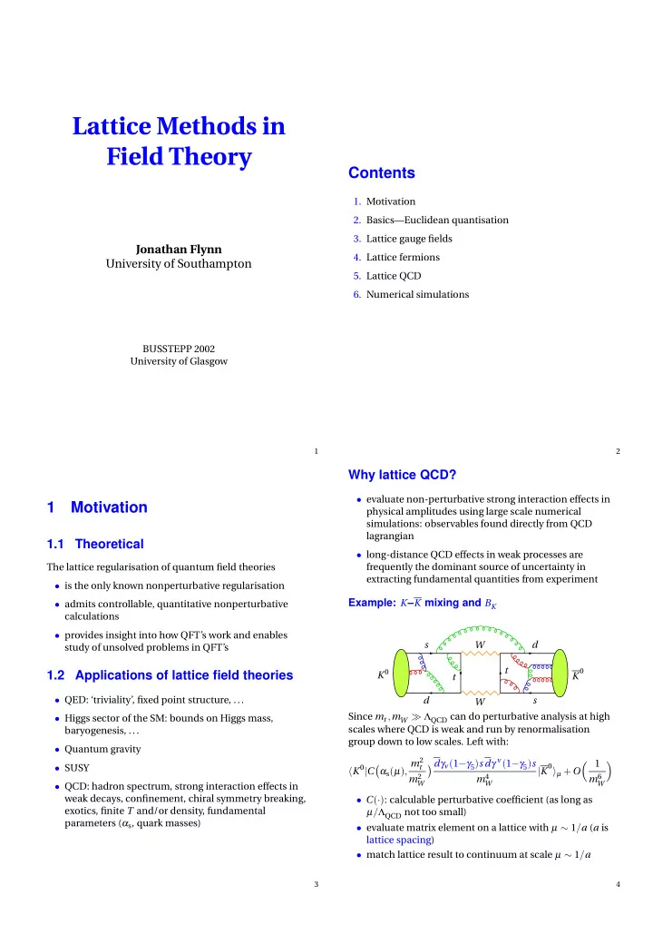is the only known nonperturbative regularisation Example: K – K mixing and B K • admits controllable, quantitative nonperturbative calculations • provides insight into how QFT’s work and enables s W d study of unsolved problems in QFT’s t K 0 K 0 1.2 Applications of lattice field theories t • QED: ‘triviality’, fixed point structure, ... d s W Since m t , m W ≫ Λ QCD can do perturbative analysis at high • Higgs sector of the SM: bounds on Higgs mass, scales where QCD is weak and run by renormalisation baryogenesis, ... group down to low scales. Left with: • Quantum gravity � 1 α s ( µ ) , m 2 � d γ ν ( 1 − γ 5 ) s d γ ν ( 1 − γ 5 ) s � | K 0 � µ + O • SUSY � K 0 | C t � m 2 m 4 m 6 W W W • QCD: hadron spectrum, strong interaction effects in weak decays, confinement, chiral symmetry breaking, • C ( · ) : calculable perturbative coefficient (as long as exotics, finite T and/or density, fundamental µ / Λ QCD not too small) parameters ( α s , quark masses) • evaluate matrix element on a lattice with µ ∼ 1 / a ( a is lattice spacing) • match lattice result to continuum at scale µ ∼ 1 / a 3 4

CKM matrix and unitarity triangle Unitarity triangle � V ud V us V ub � V ud V ∗ ub + V cd V ∗ cb + V td V ∗ tb = 0 V cd V cs V cb = V td V ts V tb 1 ∆ m s & ∆ m d 1 − λ 2 / 2 A λ 3 ( ρ − i η ) � λ � CK M ∆ m d f i t t e r + O ( λ 4 ) 1 − λ 2 / 2 A λ 2 − λ 0.8 A λ 3 ( 1 − ρ − i η ) − A λ 2 1 0.6 Unitarity: V ud V ∗ ub + V cd V ∗ cb + V td V ∗ tb = 0 η 0.4 V ud V ∗ A λ 3 ( ρ + i η ) + O ( λ 7 ) = ub | V ub /V cb | |ε K | − A λ 3 + O ( λ 7 ) 0.2 V cd V ∗ = sin 2 β WA cb V td V ∗ A λ 3 ( 1 − ρ − i η ) + O ( λ 7 ) = 0 tb -1 -0.5 0 0.5 1 where ρ = ρ ( 1 − λ 2 / 2 ) and η = η ( 1 − λ 2 / 2 ) . ρ Measurement V CKM × other Constraint 2 � � b → u V ub ρ 2 + η 2 ( ρ , η ) � � � � b → c V cb � � α | V td | 2 f 2 ( 1 − ρ ) 2 + η 2 ∆ M d B d B B d f ( m t ) 2 f 2 ρ + i η 1 − ρ − i η B d B B d � � ∆ M d V td ( 1 − ρ ) 2 + η 2 � � � � f 2 ∆ M s V ts B s B B s � � ε K f ( A , η , ρ , B K ) ∝ η ( 1 − ρ ) γ β (CKMfitter Spring 2002: H H¨ ocker et al, hep-ph/0104062; http://ckmfitter.in2p3.fr/) ( 0 , 0 ) ( 1 , 0 ) 5 6 2 Basics: Euclidean quantisation Lattice embedded in d -dimensional Euclidean spacetime Ta t ...with sin2 β from BaBar and Belle, Standard Model is in good shape. Errors in the nonperturbative parameters are now the limiting factor in more precise testing to look for effects from New Physics. La s There is also a rich upcoming experimental programme in the next few years which will need or test lattice results: a s • B -factories: constraining unitarity triangle, rare decays • Tevatron Run II: ∆ M B s , ∆Γ B s , b -hadron lifetimes, ... • CLEOc: leptonic and semileptonic D decays, masses of a t quarkonia, hybrids, glueballs a s , a t lattice spacings • LHC: ... La s length in spatial dimension(s) Ta t length in temporal dimension Matter fields live on lattice sites x . Example: scalar field x j = na s , n = 0 ,..., L − 1 φ ( x ) with x 0 = ma t , m = ,..., T − 1 7 8

2.1 Lattice as a regulator Fourier transform of a lattice scalar field in one dimension: x = na , n = 0 ,..., L − 1 , with periodic boundary conditions: L − 1 e − ipna φ ( x ) ˜ ∑ φ ( p ) = a 2.2 Euclidean quantisation on the lattice n = 0 φ ( x + La ) φ ( x ) = Path integral well-defined in Euclidean space • discretisation implies Wick Minkowski Euclidean • ˜ φ ( p ) periodic with period 2 π / a rotation • momenta lie in first Brillouin zone i ε prescription avoids poles − π a < p ≤ π a Procedure • have introduced a momentum cutoff; Λ = π 1. Continuum classical Euclidean field theory a 2. Discretisation − → lattice action • spatial periodicity implies momentum p quantised in 3. Quantisation − → functional integral units of 2 π / La • gauge invariance and gauge fields, fermions: later Lattice provides both UV and IR cutoffs. Ultimately want infinite volume ( L , T → ∞ ) and continuum ( a → 0 ) limits. Most effort devoted to continuum limit. 9 10 Step 2: Discretisation Introduce a hypercubic lattice Λ E with a t = a s = a . x 0 x 1 , 2 , 3 � � Step 1 x ∈ a Z 4 � Λ E = � a = 0 ,..., T − 1; = 0 ,..., L − 1 � a Euclidean fields φ ( x ) obtained formally from analytic • L 3 T lattice sites continuation • finite volume t → − ix 0 , φ ( x , t ) → φ ( x ) • finite number d.o.f. Action: Lattice action: � � 1 � 2 ( ∂ µ φ ) 2 + V ( φ ) d 4 x S E [ φ ] = � � S E [ φ ] = a 4 ∑ 1 2 ∇ µ φ ( x ) ∇ µ φ ( x ) + V ( φ ) where µ = 0 , 1 , 2 , 3 and x ∈ Λ E V ( φ ) = 1 2 m 2 φ 2 + λ with forward and backward lattice derivatives 4! φ 4 1 � � φ ( x + a ˆ ∇ µ φ ( x ) ≡ µ ) − φ ( x ) a Minkowski ← → Euclidean 1 ∇ ∗ � � φ ( x ) − φ ( x − a ˆ µ φ ( x ) ≡ µ ) O ( 4 ) symmetry Lorentz symmetry a t 2 − x 2 invariant ( x 0 ) 2 + x 2 invariant  +   +  Lattice Laplacian: − +         − + 3     ( ∇ ∗ ∑ ∆ φ ( x ) ≡ µ ∇ µ ) φ ( x ) − + µ = 0 3 1 � � ∑ = φ ( x + a ˆ µ ) + φ ( x − a ˆ µ ) − 2 φ ( x ) a 2 µ = 0 11 12

Step 3: Quantisation—functional integral Lattice action for a free scalar field: � D [ φ ] e − S E [ φ ] Z E ≡ � � S E [ φ ] = a 4 ∑ − 1 2 φ ( x ) ∆ φ ( x ) + V ( φ ) x ∈ Λ E D [ φ ] is the measure, eg: D [ φ ] = ∏ d φ ( x ) Remarks x ∈ Λ E • finite number of integrations • Discretisation is not unique. Can use different definitions for ∇ ( ∗ ) µ and/or V ( φ ) as long as they become Correlation functions the same in the naive continuum limit, a → 0 . � φ ( x 1 ) ··· φ ( x n ) � ≡ 1 � D [ φ ] φ ( x 1 ) ··· φ ( x n ) e − S E [ φ ] ∗ Universality: discretisations fall into classes, each Z E member of which has the same continuum limit • �·� is shorthand for � 0 | T · | 0 � , time-ordered vacuum ∗ Improvement: optimise choice of lattice action for expectation value a faster approach to the continuum limit • well-defined if S E [ φ ] > 0 • O ( 4 ) (eventually Lorentz symmetry) is not preserved. • particle spectrum implicitly determined by correlation Have cubic symmetry instead; recover O ( 4 ) symmetry functions as a → 0 . • analytically continue to Minkowski space and get S -matrix elements ( = physics) via LSZ 13 14 Lattice propagator Relation between W [ J ] and K : 2.3 Generating functional e W [ J ] = 1 � d φ ( x ) e − S E [ φ ] e ( J , φ ) = e 2 ( J , K − 1 J ) 1 ∏ Scalar product on space F of fields φ over Λ E : Z E x ∈ Λ E ( φ 1 , φ 2 ) = a 4 ∑ φ 1 ( x ) φ 2 ( x ) Diagonalise K through Fourier transform: x ∈ Λ E J ( p ) = a 4 ∑ 1 e ip · x ˜ e − ip · y J ( y ) , ˜ a 4 L 3 T ∑ J ( x ) = J ( p ) Action for free scalar field: p ∈ Λ ∗ y ∈ Λ E E S E [ φ ] = 1 Λ ∗ K = − ∇ ∗ µ ∇ µ + m 2 E is the dual lattice (or set of momentum points in the 2 ( φ , K φ ) , Brillouin zone): K is a linear operator on F . � � p 0 = 2 π p 1 , 2 , 3 = 2 π � Λ ∗ = p Ta n 0 , La n 1 , 2 , 3 ; � Let J ( x ) be an external field (source) on Λ E , J ∈ F , and E define the generating functional W [ J ] through, � n 0 = 0 ,..., T − 1 , n 1 , 2 , 3 = 0 ,..., L − 1 e W [ J ] � e ( J , φ ) � ≡ 1 � d φ ( x ) e − S E [ φ ] e ( J , φ ) ∏ = Z E x ∈ Λ E 2 π / a aT Correlation functions found by differentiating w.r.t. J ( x ) : ∂ ∂ J ( x ) e W [ J ] a 4 � φ ( x ) e ( J , φ ) � = aL 2 π / a ∂ 2 � ∂ J ( x 1 ) ∂ J ( x 2 ) e W [ J ] � ( a 4 ) 2 � φ ( x 1 ) φ ( x 2 ) � = � � J = 0 2 π / a aL Λ ∗ Λ E E 15 16