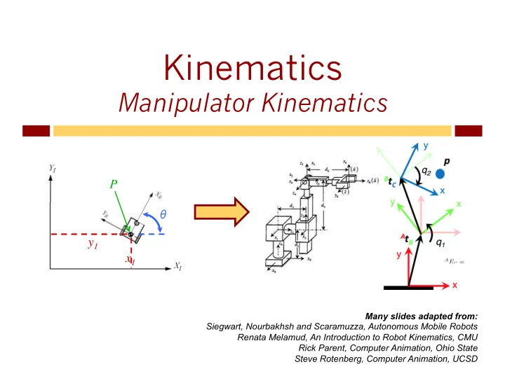
Kinematics Manipulator Kinematics P P y 1 y 1 x 1 x 1 Many - - PowerPoint PPT Presentation

kinematics
SMART_READER_LITE
LIVE PREVIEW

Kinematics Manipulator Kinematics P P y 1 y 1 x 1 x 1 Many - - PowerPoint PPT Presentation

Kinematics Manipulator Kinematics P P y 1 y 1 x 1 x 1 Many slides adapted from: Siegwart, Nourbakhsh and Scaramuzza, Autonomous Mobile Robots Renata Melamud, An Introduction to Robot Kinematics, CMU Rick Parent, Computer Animation,


slide-1
SLIDE 1

Kinematics

Manipulator Kinematics

x1 y1 P

θ

x1 y1 P

θ

Many slides adapted from: Siegwart, Nourbakhsh and Scaramuzza, Autonomous Mobile Robots Renata Melamud, An Introduction to Robot Kinematics, CMU Rick Parent, Computer Animation, Ohio State Steve Rotenberg, Computer Animation, UCSD

slide-2
SLIDE 2

2

Bookkeeping

u Homework

u Resolution, Kinematics & IK, Course Progress u Due Thursday night

u Quiz 3: Manipulation, Grasping, Kinematics

u Due tomorrow night (not Thursday)

u Assignment 3:

u Build hardware!

u Today:

u Transformations, affines u Chasles’ theorem

slide-3
SLIDE 3

3

Assignment 3

u Build LED circuit

u Breadboard-based building u Parts in lab / class Thursday

u Build motor

u Very simple conceptually

u Some of this will be in-class workshop

u 12th November u Due on 13th

slide-4
SLIDE 4

4

u Forward:

u Inputs: joint angles u Outputs: coordinates of end-effector

u Inverse:

u Inputs: desired coordinates of end-effector u Outputs: joint angles

u Inverse kinematics are tricky

u Multiple solutions u No solutions u Dead spots

Forward & Inverse

Joint space (robot space – previously R)

θ1, θ2, …, θn

Cartesian space (global space – previously I)

(x,y,z}, r/p/y

slide-5
SLIDE 5

5

u Transform between robot and world coordinates

u Why?

u Transformation of parts (points) of the robot

Actual Goal

R: {0, 0, 0} I: {4, 2, 3}

x y z

R: {0, 0, -2} I: {4, 2, 5}

slide-6
SLIDE 6

6

u Affine transformation

u Preserves collinearity (i.e., all points lying on a line initially

still lie on a line after transformation)

u Preserves ratios of distances (e.g., the midpoint of a line

segment remains the midpoint after transformation)

u Rigid transform

u Reflections, translations, rotations u Preserves internal relationship of points

u Distances between every pair of points u (Remember, this is not the robot moving!)

Actual Goal

slide-7
SLIDE 7

7

u Affine transformations: u Given a point x (x,y), transformed x’ can be written:

u Translation u Rotation u Scaling u Shear

Affine Transformations

x’ =[ ] ax + by + c dx + ey + f x’ =[ ] x+c y+f x’ =[ ] xcosθ – ysinθ xsinθ + ycosθ

slide-8
SLIDE 8

8

u These can all be done with matrix multiplication u But, this is not a linear transform

u Represent points in space using vectors u Transform using 2x2 (or 3x3) matrices

But:

u Multiplying a zero vector by a matrix gives you?

u Another zero vector

u Can’t move the origin!

Homogenous Coordinates

slide-9
SLIDE 9

9

u So we need homogenous coordinates u Add identity column/row u Translation becomes

Homogenous Coordinates

1 0 0 x 0 1 0 y 0 0 1 z 0 0 0 1 1 0 0 Δx 0 1 0 Δy 0 0 1 Δz 0 0 0 1

slide-10
SLIDE 10

10

DH Parameters

ai-1 : link length – distance Zi-1 and Zi along Xi αi-1 : link twist – angle Zi-1 and Zi around Xi di : link offset – distance Xi-1 to Xi along Zi θ2 : joint angle – angle Xi-1 and Xi around Zi

slide-11
SLIDE 11

11

Translation

ξI = xI yI zI θ ξR = xR yR zR θ Origin of R in I: 3 1 In 3D: 1 0 0 0 0 1 0 3 0 0 1 0 0 0 0 1 Generally: 1 0 0 x 0 1 0 y 0 0 1 z 0 0 0 1

slide-12
SLIDE 12

12

Rotation

ξI = x y z θI ξR = x y z θR Generally: Introduction to Homogeneous Transformations & Robot Kinematics Jennifer Kay 2005

slide-13
SLIDE 13

13

Example: Rotation in Plane

slide-14
SLIDE 14

14

ai-1 : distance Zi-1 and Zi along Xi αi-1 : angle Zi-1 and Zi around Xi di : distance Xi-1 to Xi along Zi θ2 : angle Xi-1 and Xi around Zi

u Coordinate transformation:

Transformation i to i-1 (2)

screw displacement: screw displacement:

slide-15
SLIDE 15

15

Transformation i to i-1 (3)

Transformation in DH:

slide-16
SLIDE 16

16

Inverse Kinematics

u Compute the vector of joint DOFs that will cause the end

effector to reach some desired goal state

u In other words, it is the inverse previous problem

u Analytic approach

u Directly calculate joint angles in configuration that satisfies goal

u Numeric approach

u At each time slice, determine joint movements that take you in

direction of goal position (and orientation)

  • 1. Set goal configuration of end effector
  • 2. calculate interior joint angles
slide-17
SLIDE 17

17

Goal End Effector θ1 θ2 θ3 L1 L2 L3

Inverse Kinematics

slide-18
SLIDE 18

18

Inverse Kinematics

u Undercon

erconst strain ined ed

u Fewer constraints than DoFs u Many solutions

u Overcon

erconst strain ined ed

u Too many constraints u No solution

u Rea

each chable le wor

  • rksp

space ce

u Volume the end effector can reach

u Dext

extrou rous wor

  • rksp

space ce

u Volume end effector can reach in any orientation

slide-19
SLIDE 19

19

Given arm configuration (L1, L2, …) Given desired goal position (and orientation) of end effector: [x,y,z, ψ1,ψ2, ψ3] Analytically compute goal configuration (θ1,θ2) Interpolate pose vector from initial to goal

Analytic

slide-20
SLIDE 20

20

Analytic Inverse Kinematics

(X,Y) L1 L2 θ1 θ2 Goal

slide-21
SLIDE 21

21

(X,Y) Goal Multiple solutions

Analytic Inverse Kinematics

slide-22
SLIDE 22

22

(X,Y) L1 L2 θ1 θT 180- θ2

Analytic Inverse Kinematics

slide-23
SLIDE 23

23

(X,Y) L1 L2 θ1 θT 180- θ2 X Y

x 2 + y 2

Analytic Inverse Kinematics

slide-24
SLIDE 24

24

A B C α

AB C B A 2 ) cos(

2 2 2

− + = α

Law of Cosines

slide-25
SLIDE 25

25

(X,Y) L1 L2 θ1 θT

180- θ2

X Y

x 2 + y 2

2 2

) cos( Y X X

T

+ = θ ⎟ ⎟ ⎠ ⎞ ⎜ ⎜ ⎝ ⎛ + =

− 2 2 1

cos Y X X

T

θ

2 2 1 2 2 2 2 2 1 1

2 ) cos( Y X L L Y X L

T

+ − + + = −θ θ

T

Y X L L Y X L θ θ + + − + + =

) 2 ( cos

2 2 1 2 2 2 2 2 1 1 1

( )

2 1 2 2 2 2 2 1 2

2 ) 180 cos( L L Y X L L + − + = −θ

( ))

2 ( cos 180

2 1 2 2 2 2 2 1 1 2

L L Y X L L + − + − =

θ

Analytic Inverse Kinematics

slide-26
SLIDE 26

26

Analytic Inverse Kinematics

slide-27
SLIDE 27

27

When linkage is too complex for analytic methods At each time step, determine changes to joint angles that take the end effector toward goal position and orientation Need to recompute at each time step

Iterative Inverse Kinematics

slide-28
SLIDE 28

28

End Effector θ2 a2 d2 a2 x d2 Compute instantaneous effect of each joint Linear approximation to curvilinear motion Find linear combination to take end effector towa ward rds goal position

Inverse Jacobian Method

slide-29
SLIDE 29

29

Instantaneous linear change in end effector for ith joint

Inverse Jacobian Method

slide-30
SLIDE 30

30

What is the change in

  • rientation of end effector

induced by joint i that has axis of rotation a i and position Ji?

i i

a ω =

  • Angular velocity

Inverse Jacobian Method

slide-31
SLIDE 31

31

Solution only valid for an instantaneous step Angular affect is really curved, not straight line Once a step is taken, need to recompute solution

Inverse Jacobian Method

slide-32
SLIDE 32

32

y1 = f1(x1,x2,x3,x4,x5,x6) y2 = f2(x1,x2,x3,x4,x5,x6) y3 = f3(x1,x2,x3,x4,x5,x6) y4 = f4(x1,x2,x3,x4,x5,x6) y5 = f5(x1,x2,x3,x4,x5,x6) y6 = f6(x1,x2,x3,x4,x5,x6)

Set up equations yi: state variable xi : system parameter fi : relate system parameters to state variable

Inverse Jacobian: Math

slide-33
SLIDE 33

33

y1 = f1(x1,x2,x3,x4,x5,x6) y2 = f2(x1,x2,x3,x4,x5,x6) y3 = f3(x1,x2,x3,x4,x5,x6) y4 = f4(x1,x2,x3,x4,x5,x6) y5 = f5(x1,x2,x3,x4,x5,x6) y6 = f6(x1,x2,x3,x4,x5,x6)

Matrix Form

Y = F(X)

Inverse Jacobian: Math

slide-34
SLIDE 34

34

Use chain rule to differentiate equations to relate changes in system parameters to changes in state variables

) , , , , , (

6 5 4 3 2 1 1

x x x x x x f yi =

6 6 5 5 4 4 3 3 2 2 1 1

dx x f dx x f dx x f dx x f dx x f dx x f dy

i i i i i i i

∂ ∂ ∂ ∂ ∂ ∂ ∂ ∂ ∂ ∂ ∂ ∂ + + + + + =

Inverse Jacobian: Math

slide-35
SLIDE 35

35

Y = F(X)

dX X F dY ∂ ∂ =

6 6 5 5 4 4 3 3 2 2 1 1

dx x f dx x f dx x f dx x f dx x f dx x f y

i i i i i i i

∂ ∂ ∂ ∂ ∂ ∂ ∂ ∂ ∂ ∂ ∂ ∂ ∂ + + + + + =

Matrix Form

Inverse Jacobian: Math

slide-36
SLIDE 36

36

dX X F dY ∂ ∂ =

Change in position (and

  • rientation) of end effector

Change in joint angles Linear approximation that relates change in joint angle to change in end effector position (and orientation)

Inverse Jacobian: Math

slide-37
SLIDE 37

37

dX X F dY ∂ ∂ =

⎥ ⎥ ⎥ ⎥ ⎥ ⎦ ⎤ ⎢ ⎢ ⎢ ⎢ ⎢ ⎣ ⎡ ⎥ ⎥ ⎥ ⎥ ⎥ ⎥ ⎥ ⎥ ⎥ ⎥ ⎥ ⎥ ⎥ ⎥ ⎥ ⎦ ⎤ ⎢ ⎢ ⎢ ⎢ ⎢ ⎢ ⎢ ⎢ ⎢ ⎢ ⎢ ⎢ ⎢ ⎢ ⎢ ⎣ ⎡ = ⎥ ⎥ ⎥ ⎥ ⎥ ⎥ ⎥ ⎥ ⎦ ⎤ ⎢ ⎢ ⎢ ⎢ ⎢ ⎢ ⎢ ⎢ ⎣ ⎡

n z y x z n y y y n x x x z y x z y x

a a a p p p p p p p v v v θ θ θ ∂θ ∂ ∂θ ∂ ∂θ ∂ ∂θ ∂ ∂θ ∂ ∂θ ∂ ∂θ ∂ ∂θ ∂ ∂θ ∂ ∂θ ∂ ω ω ω

… … … … … … … … … … … … …

2 1 1 1 1 1 2 1 2 1

Inverse Jacobian: Math

slide-38
SLIDE 38

38

Jacobians

u Let’s say we have a simple 2D robot arm with two 1-

DOF rotational joints:

Φ1 Φ2

  • e=[ex ey]
slide-39
SLIDE 39

39

Jacobians

u The Jacobian matrix J(e,Φ) shows how each

component of e varies wrt. each joint angle

( )

⎥ ⎥ ⎥ ⎥ ⎦ ⎤ ⎢ ⎢ ⎢ ⎢ ⎣ ⎡ ∂ ∂ ∂ ∂ ∂ ∂ ∂ ∂ =

2 1 2 1

, φ φ φ φ

y y x x

e e e e J Φ e

slide-40
SLIDE 40

40

Jacobians

u Consider what would happen if we increased φ1 by

a small amount. What would happen to e ?

φ1

  • ∂e

∂ϕ1 = ∂ex ∂ϕ1 ∂ey ∂ϕ1 ⎡ ⎣ ⎢ ⎢ ⎤ ⎦ ⎥ ⎥

slide-41
SLIDE 41

41

Jacobians

u What if we increased φ2 by a small amount?

φ2

⎦ ⎤ ⎢ ⎣ ⎡ ∂ ∂ ∂ ∂ = ∂ ∂

2 2 2

φ φ φ

y x

e e e

slide-42
SLIDE 42

42

Jacobian for a 2D Robot Arm

φ2

  • φ1

( )

⎥ ⎥ ⎥ ⎥ ⎦ ⎤ ⎢ ⎢ ⎢ ⎢ ⎣ ⎡ ∂ ∂ ∂ ∂ ∂ ∂ ∂ ∂ =

2 1 2 1

, φ φ φ φ

y y x x

e e e e J Φ e

slide-43
SLIDE 43

43

Jacobian transpose Alternate Jacobian – use goal position HAL – human arm linkage CCD Damped Least Squares

Other Numeric IK