9/24/2010 Monitoring and data filtering III. The Kalman Filter and - - PDF document

9/24/2010 1

Dias 1

Monitoring and data filtering

• III. The Kalman Filter and its relation with the
• ther methods

Advanced Herd Management Cécile Cornou, IPH

Dias 2

Before this part of the course

Compare key figures (k) with expected results

κ = θ + es + eo

Results from 2 herds 780 790 800 810 820 830 840 850 860 870 880 2 4 6 8 10 12 Quarter Gain (g) Expected Herd A Herd B

Dias 3

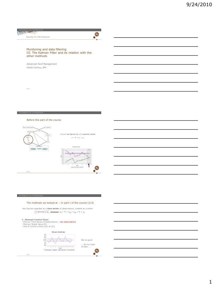
The methods we looked at – In part I of the course (1/3)

Key figures regarded as a time series of observations, treated as a whole κ = θ + es + eo κt = θ + est + eot = θ + vt I - Shewart Control Chart

• Plot our Time Series of Observations : raw observations
• Plot our Target Value (θ’)
• Plot of Control Limits (UCL & LCL)

Not so good ... for our type

• f data ...

9/24/2010 2

Dias 4

The methods we looked at – In part I of the course (2/3)

II - Shewart Control Chart

• Plot a Moving Average of our TS
• Plot our Target Value (θ’)
• Plot of Control Limits (UCL & LCL)

III - Shewart Control Chart

• Plot a EWMA of our TS
• Plot our Target Value (θ’)
• Plot of Control Limits (UCL & LCL)

Still not so good ... for our type of data Here: milk yield

Dias 5

The methods we looked at – In part I of the course (3/3)

IV – Autocorrelated data

• Model the data
• Calculate a prediction for next obs.
• Plot the prediction errors

V – EWMA for autocorrelated data

• Use EWMA as one-step-ahead

predictor

• Plot the prediction errors

Here we use 0 as Center Line and see how error terms are distributed

Dias 6

The methods we looked at – In part II of the course (1/4)

A Simple DLM Time series Yt = (y1, ... , yn) Observation equation: yt = t + vt, vt » N(0, Vt)

Like before: vt = es + eo The symbol  t is the underlying true value at time t.

System equation:  t =  t-1 + wt, wt » N(0, Wt) The true value is not any longer assumed to be constant.

Before: κt = θ + est + eot = θ + vt

9/24/2010 3

Dias 7

The methods we looked at – In part II of the course (2/4)

The Kalman Filter (t-1 | Dt-1) » N(mt-1, Ct-1) (t | Dt ) » N(mt, Ct) 1

) 1 (



  

t t t

z z  

1

) 1 (



  

t t t t t

m A Y A m

DLM and EWMA As the model adapts to the data, At converges and becomes A The calculation of the mean of the underlying level for the simple DLM looks very similar to the calculation of the EWMA

DLM EWMA

The updating equations of the Kalman Filter are used for stepwise calculation of mt and Ct

Dias 8

The methods we looked at – In part II of the course (3/4)

The different models

• Simple DLM
• DLM with a trend

General form of the DLM Observation Equation: Yt = F’t θt + νt , νt ~ N(0,Vt) System Equation: θt = Gt θt-1 + ωt, ωt ~ N(0,Wt) t = (1, … , m)’ is a vector of parameters describing the system at time t. Can include: Level, Trend, Seasonality, Periodicity, ... According to the data observed, the use of DLM allows many modeling possibilities + External information Structure

Dias 9

The methods we looked at – In part II of the course (4/4)

Monitoring methods used with DLM Monitor the forecast errors (et = Yt – ft) as we did with autocorrelated data in part I NO need for ’expected value’ V-mask Tabular cusum Can look at the different components of the models (trends, seasons)

9/24/2010 4

Dias 10

Further examples

Ex 1. Monitoring activity level A simple DLM Monitoring deviations by mean of V-mask and Tabular cusum

• Ex. 2.

Monitoring sows’ activity types in farrowing house Use of a MPKF of class I

Dias 11

Example 1. Monitoring activity level

Context Development of Group housing in EU results of Council Directive 2001/88/EEC Difficulties identifying and accessing individual sow Idea Store data in a chip and transmit info to the farmer’s PC Sensor in the chip allows to monitor activity of the sow Assumption Body Activity of sows is expected to change around the onset of oestrus Objective Develop an automated oestrus detection method for group housed sows using sows’ acceleration measurements Method Use of Dynamic Linear Models to model the sows’ activity Use of control methods that detects model deviations at the onset of oestrus

Dias 12

Outdoor facilities

9/24/2010 5

Dias 13

ACTIVITY

3 D accelerometer

The large pen

Animals and Housing

• 5 sows in group of 100
• 20 days

Activity Measurements

• Acceleration in 3 dimensions
• Four measurements per second
• Transfer PC via Blue Tooth

Video Recordings

• Four cameras used as web cam

Oestrus Detection

• Golden standard

Detect whether activity pattern changes at onset of oestrus

Dias 14

Definition of the DLM

Use hourly averages of the length of the acceleration vector Yt = acc = √ (accx

2 + accy 2 + accz 2)

Observation equation: kt = θt + vt, vt » N(0, Vt) System equation: θt = θt-1 + wt, wt » N(0, Wt) Vt = V= unknow and constant Wt = 0 (In normal condition: no change in activity) Model initialized by mean of Reference Analysis Model observations (Yt) weighted by number of observations per hour Missing observation: et=0

Dias 15

Tabular Cusum V-mask Cusum

Illustration

Model

9/24/2010 6

Dias 16

Example 2. Monitoring sows’ activity types Farrowing house

Assumption Sow’s behaviour is affected by physiological state / illness Objective Develop a method that automatically classify sows’ activity types Model selected activity types using DLM Classify each activity type using a Multi Process Kalman Filter See whether we can automatically detect the onset of farrowing Accelerometer: measured any time / during whole reproductive cycle

Dias 17

The Farrowing House

Dias 18

Data Collected – Farrowing house

Farrowing

9/24/2010 7

Dias 19

Time series and activity types

Activity types Extracts from time series of acceleration are associated to 5 activity types

• High Active (HA)
• Medium Active (MA)
• Passive Lying Side 1 (L1)
• Passive Lying Side 2 (L2)
• Passive Lying Sternally (Ls)

Learning data set: 10 minutes of each activity type Estimate the model parameters

X Y Z

3 dimensions: X,Y , Z

Dias 20

Dynamic Linear Model

Dynamic Linear Models (DLMs) combined with Kalman Filter (KF) General form of the DLM Observation Equation: Yt = F’t θt + νt , νt ~ N(0,Vt) System Equation: θt = Gt θt-1 + ωt, ωt ~ N(0,Wt) DLM combined with Kalman Filter: estimate the underlying state vector θt by its mean vector mt and its variance-covariance matrix Ct. Multivariate DLM: each observation is a 3-dimensional vector V (3 x 3) and W (3 x 3), characteristic of each activity, are estimated by EM algorithm 5 DLMs (5 activities)

           z y x Yt

Dias 21

Multi Process Kalman Filter

MPKF class I Each DLM is analysed using the updating equations of the Kalman Filter:

• One step forecast mean ft
• One step forecast variance Qt

At time t: Posterior Probabilities are estimated for each DLM

9/24/2010 8

Dias 22

Activity Classification – Farrowing

2 days before farrowing

Feeding: 7.15, 12.00, 15.30 Lying side 1 Lying side 2 Lying sternally Active

Dias 23

Activity Classification – Farrowing

Farrowing day

Lying side 1 Lying side 2 Lying sternally Active Feeding / Rooting / Nesting

Dias 24

Activity Classification – Farrowing

Percentage of activity types d-3 to d+1

9/24/2010 9

Dias 25

Activity Classification – Farrowing

Sum of 2 min HA (red), MA (orange) and Passive (blue) / hour

Cusum of HAt – HAt-24 Farrowing

Dias 26

The multi process kalman filter (MPKF) (1/2)

Multi Process Models Class I ex: Classifying sows activities in Farrowing house A single out of a range of possible DLMs is viewed as appropriate at all time for describing the entire time series Parameters : V and W  We try to find out which model is it at time t?

Dias 27

The multi process kalman filter (MPKF) (2/2)

Multi Process Models Class II ex: Monitoring Somatic Cell Counts / Boar visits No single DLM as adequate for all time: the possibility that different models are appropriate at different times is explicitly recognised and modelled through different defining parameters Parameters : V and W and Π (values for Π define fixed prior probabilities)  We try to find out normal evolution, outlier, level shift  We need to go back f.x. two, three steps to check which model is the right one

9/24/2010 10

Dias 28

Sum up of sum up

We increased the complexity of our models and monitoring methods to try to adapt to the complexity of monitoring living beings Methods here based on a whole time series of observations

• > need for automatic registration
• > potential on-line monitoring

From part I to part II, we made our model dynamics, so the ’true underlying level’ is no more constant