Kinematics Manipulator Kinematics P P y 1 y 1 x 1 x 1 Many - PowerPoint PPT Presentation

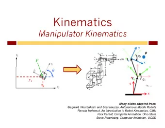
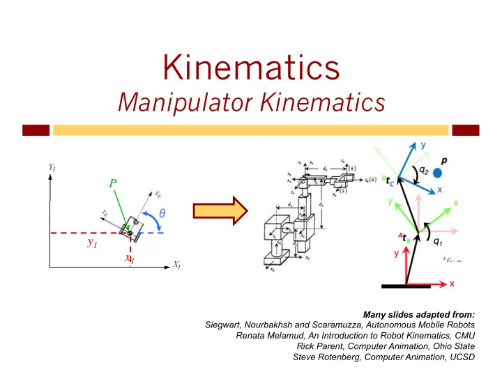
Kinematics Manipulator Kinematics P P θ θ y 1 y 1 x 1 x 1 Many slides adapted from: Siegwart, Nourbakhsh and Scaramuzza, Autonomous Mobile Robots Renata Melamud, An Introduction to Robot Kinematics, CMU Rick Parent, Computer Animation, Ohio State Steve Rotenberg, Computer Animation, UCSD

Bookkeeping 2 u Upcoming: u Projects: u Wiki permissions – http://tiny.cc/robotics-team-schedules u Posted tonight: u Quiz 3: Manipulation, Grasping, Kinematics u Con oncep cepts! s! u Homework 2 u Resolution, Kinematics & IK, Course Progress u Today: Inverse kinematics

Forward & Inverse 3 Joint space (robot u Forward: space – previously R ) u Inputs: joint angles θ 1 , θ 2 , … , θ n u Outputs: coordinates of end-effector u Inverse: u Inputs: desired coordinates of end-effector u Outputs: joint angles u Inverse kinematics are tricky u Multiple solutions u No solutions (x,y,z}, r/p/y u Dead spots Cartesian space (global space – previously I )

Forward Kinematics 4 u We will sometimes use the vector Φ to represent the array of M joint values: [ ] Φ ... = φ φ φ 1 2 M u We will sometimes use the vector e to represent an array of N joint values that describe the end effector in world space: ⎡ ⎤ e = e 1 e 2 ... e N ⎣ ⎦ u Example: u If our end effector is a full joint with orientation, e would contain 6 DOFs: 3 translations and 3 rotations. If we were only concerned with the end effector position, e would just contain the 3 translations.

Describing A Manipulator 5 u Arm made up of links in a chain u How to describe each link? u Many choices exist u DH parameters widely used u Although it’s not true that quaternions are not widely used u Joints each have coordinate system u {x,y,z}, r/p/y — OR!! joint i+1 u DH parameters u Denavit-Hartenberg joint i joint i-1 u a i-1 , α i-1 , d i , θ 2

DH Parameters 6 a i-1 : link length – distance Z i-1 and Z i along X i � α i-1 : link twist – angle Z i-1 and Z i around X i d i : link offset – distance X i-1 to X i along Z i � θ 2 : joint angle – angle X i-1 and X i around Z i

Forward: i à i-1 7 u We are we looking for: Transformation matrix T going from i to i-1: i-1 i-1 T i (or T ) i u Determine position and orientation of end-effector as function of displacements in joints u Why? u We can multiply out along all joints

Translation 8 x I x R y I y R ξ R = ξ I = z I z R θ θ Origin of R in I: In 3D: Generally: 0 1 0 0 0 1 0 0 x 3 0 1 0 3 0 1 0 y 0 0 0 1 0 0 0 1 z 1 0 0 0 1 0 0 0 1

Rotation 9 x x y y ξ I = ξ R = z z θ I θ R Generally: Review? Introduction to Homogeneous Transformations & Robot Kinematics Jennifer Kay 2005

Example: Rotation in Plane 10

Transformation i to i-1 (2) 11 a i-1 : distance Z i-1 and Z i along X i � screw α i-1 : angle Z i-1 and Z i around X i displacement: d i : distance X i-1 to X i along Z i � screw θ 2 : angle X i-1 and X i around Z i displacement: u Coordinate transformation:

Transformation i to i-1 (3) 12 Transformation in DH:

Inverse Kinematics 13 u Goal: u Compute the vector of joint DOFs that will cause the end effector to reach some desired goal state u In other words, it is the inverse previous problem u Instead of function from world space to robot space. ( ) e f Φ 1 ( ) Φ = f e − = ßà

Inverse Kinematics Issues 14 u IK is challenging! u f () is (usually) relatively easy to evaluate u f -1 () usually isn’t u Issues: u There may be several possible solutions for Φ u There may be no solutions u If there is a solution, it may be expensive to find it u There are some local-minimum “stuck” configurations u Many different approaches to solving IK problems

Analytical vs. Numerical 15 u One major way to classify IK-solving approaches: � analyt ytica ical vs numer merica ical methods u Analytical u Find an exact solution by directly inverting the forward kinematics equations. u Works on relatively simple chains. u Numerical u Use approximation and iteration to converge on a solution. u More expensive, more general purpose. u We will look at one technique: Jacobians

Calculus Review Review adapted from: Steve Rotenberg, Computer Animation, UCSD http://graphics.ucsd.edu/courses/cse169_w05

Derivative of a Scalar Function 17 u If we have a scalar function f of a single variable x, we can write it as f(x) u Derivative of function with respect to x is df/dx u The derivative is defined as: ( ) ( ) df f f x x f x Δ + Δ − lim lim = = dx x x x 0 x 0 Δ Δ Δ → Δ →

Derivative of a Scalar Function 18 f(x) Slope=df/dx f-axis x-axis x

Derivative of f(x)=x 2 19 2 ( ) For example : f x x = ( ) ( ) f x x f x + Δ − 2 2 ( ) ( ) df x x x lim + Δ − = lim = x x 0 Δ Δ → dx x x 0 Δ Δ → 2 2 2 x 2 x x x x + Δ + Δ − lim = x x 0 Δ Δ → 2 2 x x x Δ + Δ lim = x x 0 Δ Δ → ( ) lim 2 x x 2 x = + Δ = x 0 Δ →

Exact vs. Approximate 20 u Many algorithms require the computation of derivatives u Sometimes, we can compute them. For example: df 2 ( ) f x x 2 x = = dx u Sometimes function is complex, can’t compute an exact derivative u As long as we can evaluate the function, we can always approximate a derivative ( ) ( ) df f x x f x + Δ − for small x ≈ Δ dx x Δ

Approximate Derivative 21 f(x) f(x+ Δ x) Slope= Δ f/ Δ x f-axis x-axis Δ x

Nearby Function Values 22 u If we know the value of a function and its derivative at some x, we can estimate what the value of the function is at other points near x f df Δ ≈ x dx Δ df f x Δ ≈ Δ dx df ( ) ( ) f x x f x x + Δ ≈ + Δ dx

Finding Solutions to f(x)=0 23 u There are many mathematical and computational approaches to finding values of x for which f(x)=0 u One such way is the gradient descent method u If we can evaluate f(x) and df/dx for any value of x, we can always follow the gradient (slope) in the direction (currently) headed towards 0

Gradient Descent 24 u We want to find the value of x that causes f(x) to equal 0 u We will start at some value x 0 and keep taking small steps: x i+1 = x i + Δ x until we find a value x N that satisfies f(x N )=0 u For each step, (try to) choose a value of Δ x that gets closer to our goal u Use the derivative as approximation of slope of function u Use this to move ‘downhill’ towards zero

Gradient Descent 25 df/dx f(x i ) f-axis x i x-axis

Minimization 26 u If f(x i ) is not 0, the value of f(x i ) can be thought of as an error u Goal of gradient descent: minimize this error u Making it a member of the class min minimiza imization ion alg lgor orit ithms ms u Each step Δ x results in function changing its value u Call this Δ f u Ideally, Δ f = -f(x i ) – in other words, want to take a step Δ x that causes Δ f to cancel out the error u Realistically, hope each step brings us closer, and we can eventually stop when we get close enough u This iterative process is consistent with numerical algorithms

Choosing Δ x Step 27 u Safety vs. efficiency u If step size is too small, converges very slowly u If step size is too large, algorithm not reduce f. u Because the first order approximation is valid only locally. u If function varies widely, what is safest? u If we have a relatively smooth function? u If we feel very confident? u We could try stepping directly to where linear approximation passes through 0