Inverse kinematics Forward kinematics Given a joint configuration, - - PowerPoint PPT Presentation

Inverse kinematics

Kinematics

The study of motion without regard to the forces that cause it Forward kinematics

Given a joint configuration, what is the position of an end point on the structure?

Inverse kinematics

Given the position for an end point on the structure, what angles do the joints need to be to achieve that end point?

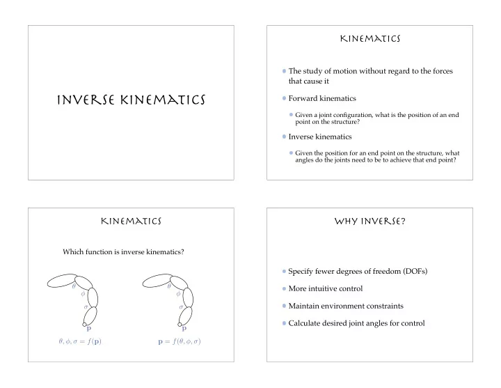
Kinematics

p θ φ σ θ, φ, σ = f(p) p θ φ σ p = f(θ, φ, σ) Which function is inverse kinematics?

Why inverse?

Specify fewer degrees of freedom (DOFs) More intuitive control Maintain environment constraints Calculate desired joint angles for control

An interactive IK system

Create a handle on the character Interactively pull the handle around IK system figures out the appropriate the joint configurations

Joint configurations

q = x, y, z, θpelvis, φpelvis, σpelvis, θthigh, φthigh, σthigh, θknee, . . .

θpelvis, φpelvis, σpelvis θthigh, φthigh, σthigh θknee θankle, φankle

Constraints

Position constraint Orientation constraint

C(q) = h(q) − p = 0 C(q) = d(q) − v = 0

h(q) p

Solutions

Closed form solutions can only be found for fairly simple mechanisms Numerical solutions

No solution Single solution Multiple solution

Under-specified problem

Multiple solutions

Mostly bad

How do we find the optimal solution?

Heuristics (move the outermost links first) Closest to the current configuration Energy minimization Natural looking motion (whatever it means)

Ik methods

Iterative methods Optimization methods

Unconstrained optimization Constrained optimization

Iterative method

Use inverse of Jacobian to iteratively step all the joint angles towards the goal Girard and Maciejewski, Computational modeling for the computer animation of legged figures, SIGGRAPH 85

Jacobian matrix

DOF (n) Constraint (m)

∂Ci ∂qj

i j

Jacobian is a m by n matrix that relating differential changes of to changes of

q C

Jacobian maps the velocity in state space to velocities in Cartesian space Jacobian depends on current state

IK and the Jacobian

J = ∂C ∂q ∂C = J∂q ∂q = J−1∂C qnew = q + ∆tJ−1∂C Linearize about current q

Invert Jacobian

But Jacobian is most likely non-square Compute the pseudo inverse Jacobian J+

∂C = J∂q JT ∂C = JT J∂q (JT J)−1JT ∂C = (JT J)−1JT J∂q J+∂C = ∂q J+ = (JT J)−1JT = JT (JJT )−1

Optimization method

Find a solution that optimizes some numeric metric and satisfies constraints Numeric metric

A function of q that measures the quantity to be minimized Also called “objective function”

Optimization method

min

q G(q)

C(q) = 0 subject to Solve for joint configuration q

Objective functions

Joint velocity Power consumption Similarity to the rest pose Similarity to the natural pose

Constraint Derivatives

What do we want?

A direction to move joints in such way that the constraint handles move towards the goal

What do derivatives tell us?

A direction constraint handles move if joints move

Constraint derivatives

∂C(q) ∂q = ∂h(q) ∂q

h(q) p

x, y, z, θ0, φ0, σ0 θ1 θ2, φ2 q = [x, y, z, θ0, φ0, σ0, θ1, θ2, φ2]

C(q) = h(q) − p = 0

Need to know how to compute derivatives for each transformation

∂h(q) ∂θ1 = T(x, y, z)R(θ0, φ0, σ0)T∂R(θ1) ∂θ1 TR(θ2, φ2)hk h(q) = T(x, y, z)R(θ0, φ0, σ0)TR(θ1)TR(θ2, φ2)hk hk: local coordinate of h

Constraint derivatives

h(q) p

x, y, z, θ0, φ0, σ0 θ1 θ2, φ2

h(q) = T(x, y, z)R(θ0, φ0, σ0)TR(θ1)TR(θ2, φ2)hk hk: local coordinate of h

What is the most efficient way to compute the ?

∂h(q) ∂q

Unconstrained Optimization

Treat each constraint as a separate metric and minimize weighted sum of all metrics Also called penalty methods

each spring pulls on constraint with force proportional to violation of the constraint

Unconstrained optimization

Minimize F(q) = G(q) +

• i

wiCi(q)2 Move in the direction of −∂F ∂q = −∂G ∂q − 2

• i

wi ∂Ci ∂q Ci Update the state qnew = q − α∂F ∂q

Search and step

Find direction and the step size that move joints closer to constraints Step size: where min

α F(q + α∆q)

α

Direction: ∆q = −∂F

∂q

qnew = q + α∆q

Unconstrained optimization

Pros:

simple and fast, no linear system to solve near-singular configurations is less of a problem

Cons:

constraints fight against each other and the objective function can’t maintain constraints exactly linear convergence

Constrained optimization

Solve a linear system comprised of Jacobians and the quadratic metric Also called Lagrangian Multipliers

L(q, λ) = G(q) − λ · C min

q,λ L(q, λ)

Constrained method

Pros

Enforce constraints exactly Quadratic convergence

Cons

Large system of equations Near-singular configurations cause instability