Joint Signal Analysis Overview Introduction Mostly we have focused - - PowerPoint PPT Presentation

joint signal analysis overview introduction mostly we
SMART_READER_LITE
LIVE PREVIEW

Joint Signal Analysis Overview Introduction Mostly we have focused - - PowerPoint PPT Presentation

Joint Signal Analysis Overview Introduction Mostly we have focused on estimating statistical properties of a Cross-correlation single univariate signal Cross Power Spectrum Autocorrelation function (ACF) Examples Partial


slide-1
SLIDE 1

System Identification
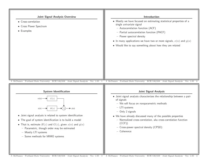
w(n) x(n) y(n)

G(z) H(z) Σ

  • Joint signal analysis is related to system identification
  • The goal of system identification is to build a model
  • That is, estimate H(z) and G(z), given x(n) and y(n)

– Parametric, though order may be estimated – Mostly LTI systems – Some methods for MIMO systems

  • J. McNames

Portland State University ECE 538/638 Joint Signal Analysis

  • Ver. 1.05

3

Joint Signal Analysis Overview

  • Cross-correlation
  • Cross Power Spectrum
  • Examples
  • J. McNames

Portland State University ECE 538/638 Joint Signal Analysis

  • Ver. 1.05

1

Joint Signal Analysis

  • Joint signal analysis characterizes the relationship between a pair
  • f signals

– We will focus on nonparametric methods – LTI systems – Only 2 signals

  • We have already discussed many of the possible properties

– Normalized cross-correlation, aka cross-correlation function (CCF)) – Cross-power spectral density (CPSD) – Coherence

  • J. McNames

Portland State University ECE 538/638 Joint Signal Analysis

  • Ver. 1.05

4

Introduction

  • Mostly we have focused on estimating statistical properties of a

single univariate signal – Autocorrelation function (ACF) – Partial autocorrelation function (PACF) – Power spectral density

  • In many applications we have two or more signals, x(n) and y(n)
  • Would like to say something about how they are related
  • J. McNames

Portland State University ECE 538/638 Joint Signal Analysis

  • Ver. 1.05

2

slide-2
SLIDE 2

Normalized Cross-Correlation Defined Normalized Cross-Correlation, also known as the Cross-correlation Function (CCF) is defined for a WSS signal as ρyx(ℓ) = γyx(ℓ)

  • γy(0)γx(0)

= γyx(ℓ) σyσx where γyx(ℓ) is the cross-covariance of y(n) and x(n), γyx(ℓ) = E [(y(n + ℓ) − µy)(x(n) − µx)∗]

  • J. McNames

Portland State University ECE 538/638 Joint Signal Analysis

  • Ver. 1.05

7

Joint Signal Analysis

w(n) x(n) y(n)

G(z) H(z) Σ

  • If we assume that x(n) and y(n) are related by an LTI system

H(z), then we can estimate the properties of H(z) given realizations of x(n) and y(n) – Magnitude – Phase – Group delay – Impulse response

  • J. McNames

Portland State University ECE 538/638 Joint Signal Analysis

  • Ver. 1.05

5

Estimated Cross-Covariance ˆ γu(ℓ)

  • 1

N − |ℓ|

N−1−|ℓ|

  • n=0

[y(n + |ℓ|) − ˆ µy] [x(n) − ˆ µx] ˆ γb(ℓ)

  • N − |ℓ|

N ˆ γu(ℓ) = 1 N

N−1−|ℓ|

  • n=0

[y(n + |ℓ|) − ˆ µy] [x(n) − ˆ µx] for |ℓ| < N. ˆ γu(ℓ) = ˆ γb(ℓ) = 0 for |ℓ| ≥ N.

  • There are similar trade-offs between biased and unbiased estimates
  • f the CCF as there were for the ACF
  • As with ACF, we generally assume the means are zero to simplify

calculations and eliminate DC artifacts

  • The bias caused by estimating the means is usually negligible
  • J. McNames

Portland State University ECE 538/638 Joint Signal Analysis

  • Ver. 1.05

8

Causality

  • Strictly speaking, given only realizations of x(n) and y(n) we

cannot determine whether one signal caused the other or not

  • This is a fundamental idea rooted in statistics
  • However, under certain assumptions causality can be determined
  • For example, if we assume that any system that relates x(n) to

y(n) or vice versa is causal, then we may be able to get a sense of which caused which from the estimated cross-correlation

  • J. McNames

Portland State University ECE 538/638 Joint Signal Analysis

  • Ver. 1.05

6

slide-3
SLIDE 3

Example 1: CCF Estimation Estimate the CCF of the ARMA process investigated earlier for PSD estimation.

  • J. McNames

Portland State University ECE 538/638 Joint Signal Analysis

  • Ver. 1.05

11

Estimated Cross-Covariance: Biased versus Unbiased If µy = µx = 0, ˆ γu(ℓ) = 1 N − |ℓ|

N−1−|ℓ|

  • n=0

y(n + |ℓ|)x(n) ˆ γb(ℓ) = 1 N

N−1−|ℓ|

  • n=0

y(n + |ℓ|)x(n)

  • The true CCF is not positive definite and the cross-spectral density

is not non-negative, in general, so this is no longer a concern

  • Nonetheless, the unbiased estimator contains excessive variance at

large lags and thus the biased estimate is generally preferred

  • J. McNames

Portland State University ECE 538/638 Joint Signal Analysis

  • Ver. 1.05

9

Example 2: MATLAB Code

L = 200; % Length of autocorrelation calculated N = 250; cl = 99; % Confidence level NP = norminv((1-cl/100)/2); % Find corresponding lower percentile of Normal b = poly([-0.8,0.97*exp(j *pi/4),0.97*exp(-j *pi/4),... 0.97*exp(j *pi/6),0.97*exp(-j *pi/6)]); % Numerator a = poly([ 0.8,0.95*exp(j*3*pi/4),0.95*exp(-j*3*pi/4),... 0.95*exp(j*2.5*pi/4),0.95*exp(-j*2.5*pi/4)]); % Denominator b = b*sum(a)/sum(b); % Set DC gain to 1 x = randn(N,1); y = filter(1,a,x);

  • J. McNames

Portland State University ECE 538/638 Joint Signal Analysis

  • Ver. 1.05

12

Estimated Cross-Correlation Functions The natural estimators of the CCF are ˆ ρb(ℓ) ˆ γb(ℓ) ˆ σxˆ σy ˆ ρu(ℓ) ˆ γu(ℓ) ˆ σxˆ σy

  • In general, it is not possible to obtain confidence intervals for the

estimated CCF because the variance of the estimator depends on the true CCF and signal ACF’s

  • Instead, it is common practice to plot the confidence intervals of a

purely random process

  • If N is large enough, the central limit theorem applies and

var{ˆ ρb(ℓ)} is approximately normal for all ℓ

  • In this case, we can use the Normal cdf to plot confidence

intervals of an IID sequence

  • These are proportional to ±
  • var{ˆ

ρyx(ℓ)}

  • This is the same as it was for the ACF
  • J. McNames

Portland State University ECE 538/638 Joint Signal Analysis

  • Ver. 1.05

10

slide-4
SLIDE 4

Example 2: Signals

20 40 60 80 100 120 140 160 180 200 −2 2 x(n) N=250 20 40 60 80 100 120 140 160 180 200 −10 −5 5 y(n) Sample (n)

  • J. McNames

Portland State University ECE 538/638 Joint Signal Analysis

  • Ver. 1.05

15

Example 2: Pole Zero Map of ARMA Process

−1 −0.5 0.5 1 −1 −0.5 0.5 1

  • J. McNames

Portland State University ECE 538/638 Joint Signal Analysis

  • Ver. 1.05

13

Example 2: MATLAB Code

figure n = 0:min(200,N); subplot(2,1,1); h = stem(n,x(n+1)); set(h(1),’MarkerFaceColor’,’b’); set(h(1),’MarkerSize’,2); xlim([0 max(n)]); ylim([min(x) max(x)]); ylabel(’x(n)’); title(sprintf(’N=%d’,N)); box off; subplot(2,1,2); h = stem(n,y(n+1),’g’); set(h(1),’MarkerFaceColor’,’g’); set(h(1),’MarkerSize’,2); xlim([0 max(n)]); ylim([min(y) max(y)]); ylabel(’y(n)’); xlabel(’Sample (n)’); box off;

  • J. McNames

Portland State University ECE 538/638 Joint Signal Analysis

  • Ver. 1.05

16

Example 2: MATLAB Code

figure h = circle; z = roots(b); p = roots(a); hold on; h2 = plot(real(z),imag(z),’bo’,real(p),imag(p),’rx’); hold off; axis square; xlim([-1.1 1.1]); ylim([-1.1 1.1]); box off;

  • J. McNames

Portland State University ECE 538/638 Joint Signal Analysis

  • Ver. 1.05

14

slide-5
SLIDE 5

Example 2: Unbiased CCF

−200 −150 −100 −50 50 100 150 200 −1 −0.8 −0.6 −0.4 −0.2 0.2 0.4 0.6 0.8 1 ρ(l) Lag (l) N=250

  • J. McNames

Portland State University ECE 538/638 Joint Signal Analysis

  • Ver. 1.05

19

Example 2: Biased CCF

−200 −150 −100 −50 50 100 150 200 −1 −0.8 −0.6 −0.4 −0.2 0.2 0.4 0.6 0.8 1 ρ(l) Lag (l) N=250

  • J. McNames

Portland State University ECE 538/638 Joint Signal Analysis

  • Ver. 1.05

17

Example 2: MATLAB Code

np = 2^nextpow2(2*N-1); % Figure out how much to pad the signal Y = fft(y,np); X = fft(x,np); cp = ifft(Y.*conj(X)); cc = real([cp(np-(L-1:-1:0));cp(1:L+1)]); cc = cc/(std(y)*std(x)); l = (-L:L).’; cc = cc./(N-abs(l)); figure h = stem(l,cc); set(h(1),’Marker’,’None’); xlim([-L L]); ylim([-1 1]); hold on; plot(l,NP*1./sqrt(N-abs(l)),’k:’,l,-NP*1./sqrt(N-abs(l)),’k:’); hold off; ylabel(’\rho(l)’); xlabel(’Lag (l)’); title(sprintf(’N=%d’,N)); box off;

  • J. McNames

Portland State University ECE 538/638 Joint Signal Analysis

  • Ver. 1.05

20

Example 2: MATLAB Code

np = 2^nextpow2(2*N-1); % Figure out how much to pad the signal Y = fft(y,np); X = fft(x,np); cp = ifft(Y.*conj(X)); cc = real([cp(np-(L-1:-1:0));cp(1:L+1)]); cc = cc/(std(y)*std(x)); cc = cc/N; l = (-L:L).’; figure h = stem(l,cc); set(h(1),’Marker’,’None’); xlim([-L L]); ylim([-1 1]); hold on; plot(xlim,NP*[1 1]/sqrt(N),’k:’,xlim,-NP*[1 1]/sqrt(N),’k:’); plot([ 0 L],[1 (N-L)/N],’g’,[ 0 L],-[1 (N-L)/N],’g’); plot([-L 0],[(N-L)/N 1],’g’,[-L 0],-[(N-L)/N 1],’g’); hold off; ylabel(’\rho(l)’); xlabel(’Lag (l)’); title(sprintf(’N=%d’,N)); box off;

  • J. McNames

Portland State University ECE 538/638 Joint Signal Analysis

  • Ver. 1.05

18

slide-6
SLIDE 6

Estimating Frequency Response

x(n) y(n) H(z)

y(n) = h(n) ∗ x(n) ryx(ℓ) = h(ℓ) ∗ rx(ℓ) Ryx(ejω) = H(ejω)Rx(ejω) H(ejω) = Ryx(ejω) Rx(ejω)

  • If x(n) and y(n) are the input and output of a system, we can use

these techniques to estimate properties of the system H(z)

  • Unlike the univariate case, if we know both x(n) and y(n) there is

no ambiguity between minimum-phase and non-minimum phase systems

  • Note that although we may be able to estimate H(ejω), this does

not mean we have a parametric description of it

  • J. McNames

Portland State University ECE 538/638 Joint Signal Analysis

  • Ver. 1.05

23

Cross-Power Spectral Density Recall that the cross-power spectral density (CPSD) is defined as Ryx(ejω)

  • ℓ=−∞

ryx(ℓ)e−jωℓ

  • Unlike the PSD, the CPSD is a complex-valued function
  • Can work with CPSD in either rectangular or polar form
  • Rectangular

– Cospectrum: Cyx(ω) Re{Ryx(ejω)} – Quadrature spectrum: Qyx(ω) Im{Ryx(ejω)}

  • More commonly, it is expressed in terms of magnitude and phase

– Cross-Amplitude Spectrum: Ayx(ω) |Ryx(ejω)| – Phase Spectrum: Φyx(ω) ∡Ryx(ejω)

  • J. McNames

Portland State University ECE 538/638 Joint Signal Analysis

  • Ver. 1.05

21

Which CPSD Estimate?

  • The book argues that Welch’s approach to modified periodogram

averaging is preferred

  • Not clear to me why they prefer this to Blackman-Tukey, which I

think is better

  • J. McNames

Portland State University ECE 538/638 Joint Signal Analysis

  • Ver. 1.05

24

Estimating Cross-Power Spectral Density The Cross-periodogram is defined as ˆ Ryx(ejω)

  • N−1
  • ℓ=−(N−1)

ˆ ryx(ℓ)e−jω = 1 N N−1

  • n=0

x(n)e−jωn N−1

  • n=0

y(n)e−jωn ∗

  • We may use the same nonparametric techniques to estimate the

CPSD that we used to estimate the PSD

  • The same tradeoffs exist

– Main lobe width versus side lobe height – Bias versus variance

  • Can reduce variance at the expense of bias using either smoothing

(Blackman-Tukey) or averaging (Welch-Bartlett)

  • J. McNames

Portland State University ECE 538/638 Joint Signal Analysis

  • Ver. 1.05

22

slide-7
SLIDE 7

Example 3: Blackman-Tukey Estimate Rx(ejω)

0.05 0.1 0.15 0.2 0.25 0.3 0.35 0.4 0.45 0.5 0.5 1 1.5 2 Estimated Rx(ejω) N:1000 L:251 NA:1000 SNR:10.0 Confidence Bands:95% True PSD Confidence Bands Average Estimate Single Estimate 0.05 0.1 0.15 0.2 0.25 0.3 0.35 0.4 0.45 0.5 10 Estimated Rx(ejω) Frequency (cycles/sample)

  • J. McNames

Portland State University ECE 538/638 Joint Signal Analysis

  • Ver. 1.05

27

Additive Noise

v(n) w(n) x(n) y(n) H(z) Σ

Ryx(ejω) = Rvx(ejω) H(ejω) = Rvx(ejω) Rx(ejω) = Ryx(ejω) Rx(ejω) Ry(ejω) = Rv(ejω) + Rw(ejω) Rv(ejω) = |H(ejω)|2Rx(ejω)

  • It is instructive to consider the case of additive noise
  • Here we assume that w(n) is statistically independent of x(n) and

all signals are stationary with zero mean

  • Note: different notation than text
  • J. McNames

Portland State University ECE 538/638 Joint Signal Analysis

  • Ver. 1.05

25

Example 3: Blackman-Tukey Estimate Ryx(ejω)

0.05 0.1 0.15 0.2 0.25 0.3 0.35 0.4 0.45 0.5 −500 500 N:1000 L:251 NA:1000 SNR:10.0 Confidence Bands:95% Real CPSD True Cross−PSD Confidence Bands Average Estimate Single Estimate 0.05 0.1 0.15 0.2 0.25 0.3 0.35 0.4 0.45 0.5 −200 200 400 Frequency (cycles/sample) Imaginary CPSD

  • J. McNames

Portland State University ECE 538/638 Joint Signal Analysis

  • Ver. 1.05

28

Example 3: Blackman-Tukey Estimate

v(n) w(n) x(n) y(n) H(z) Σ

Use the Blackman-Tukey estimate to estimate the PSDs of x(n) and y(n) for various signal to noise ratios (SNRs). Also estimate the transfer function magnitude and phase for the PZ system described earlier.

  • J. McNames

Portland State University ECE 538/638 Joint Signal Analysis

  • Ver. 1.05

26

slide-8
SLIDE 8

Example 3: Blackman-Tukey Estimate ∠H(ejω)

0.05 0.1 0.15 0.2 0.25 0.3 0.35 0.4 0.45 0.5 −150 −100 −50 50 100 150 PSD N:1000 L:251 NA:1000 SNR:10.0 Confidence Bands:95% True H Confidence Bands Average Estimate Single Estimate

  • J. McNames

Portland State University ECE 538/638 Joint Signal Analysis

  • Ver. 1.05

31

Example 3: Blackman-Tukey Estimate Ry(ejω)

0.05 0.1 0.15 0.2 0.25 0.3 0.35 0.4 0.45 0.5 1 2 3 4 5 x 10 5 Estimated Ry(ejω) N:1000 L:251 NA:1000 SNR:10.0 Confidence Bands:95% True PSD Confidence Bands Average Estimate Single Estimate 0.05 0.1 0.15 0.2 0.25 0.3 0.35 0.4 0.45 0.5 10 4 10 6 Estimated Ry(ejω) Frequency (cycles/sample)

  • J. McNames

Portland State University ECE 538/638 Joint Signal Analysis

  • Ver. 1.05

29

Example 3: Blackman-Tukey Estimate Rx(ejω)

0.05 0.1 0.15 0.2 0.25 0.3 0.35 0.4 0.45 0.5 0.5 1 1.5 2 Estimated Rx(ejω) N:1000 L:251 NA:1000 SNR:1.0 Confidence Bands:95% True PSD Confidence Bands Average Estimate Single Estimate 0.05 0.1 0.15 0.2 0.25 0.3 0.35 0.4 0.45 0.5 10 Estimated Rx(ejω) Frequency (cycles/sample)

  • J. McNames

Portland State University ECE 538/638 Joint Signal Analysis

  • Ver. 1.05

32

Example 3: Blackman-Tukey Estimate |H(ejω)|

0.05 0.1 0.15 0.2 0.25 0.3 0.35 0.4 0.45 0.5 200 400 600 800 |H(ejω)| N:1000 L:251 NA:1000 SNR:10.0 Confidence Bands:95% True H Confidence Bands Average Estimate Single Estimate 0.05 0.1 0.15 0.2 0.25 0.3 0.35 0.4 0.45 0.5 10 |H(ejω)| Frequency (cycles/sample)

  • J. McNames

Portland State University ECE 538/638 Joint Signal Analysis

  • Ver. 1.05

30

slide-9
SLIDE 9

Example 3: Blackman-Tukey Estimate |H(ejω)|

0.05 0.1 0.15 0.2 0.25 0.3 0.35 0.4 0.45 0.5 200 400 600 800 |H(ejω)| N:1000 L:251 NA:1000 SNR:1.0 Confidence Bands:95% True H Confidence Bands Average Estimate Single Estimate 0.05 0.1 0.15 0.2 0.25 0.3 0.35 0.4 0.45 0.5 10 |H(ejω)| Frequency (cycles/sample)

  • J. McNames

Portland State University ECE 538/638 Joint Signal Analysis

  • Ver. 1.05

35

Example 3: Blackman-Tukey Estimate Ryx(ejω)

0.05 0.1 0.15 0.2 0.25 0.3 0.35 0.4 0.45 0.5 −500 500 N:1000 L:251 NA:1000 SNR:1.0 Confidence Bands:95% Real CPSD True Cross−PSD Confidence Bands Average Estimate Single Estimate 0.05 0.1 0.15 0.2 0.25 0.3 0.35 0.4 0.45 0.5 −200 200 400 Frequency (cycles/sample) Imaginary CPSD

  • J. McNames

Portland State University ECE 538/638 Joint Signal Analysis

  • Ver. 1.05

33

Example 3: Blackman-Tukey Estimate ∠H(ejω)

0.05 0.1 0.15 0.2 0.25 0.3 0.35 0.4 0.45 0.5 −150 −100 −50 50 100 150 PSD N:1000 L:251 NA:1000 SNR:1.0 Confidence Bands:95% True H Confidence Bands Average Estimate Single Estimate

  • J. McNames

Portland State University ECE 538/638 Joint Signal Analysis

  • Ver. 1.05

36

Example 3: Blackman-Tukey Estimate Ry(ejω)

0.05 0.1 0.15 0.2 0.25 0.3 0.35 0.4 0.45 0.5 2 4 6 x 10 5 Estimated Ry(ejω) N:1000 L:251 NA:1000 SNR:1.0 Confidence Bands:95% True PSD Confidence Bands Average Estimate Single Estimate 0.05 0.1 0.15 0.2 0.25 0.3 0.35 0.4 0.45 0.5 10 4 10 6 Estimated Ry(ejω) Frequency (cycles/sample)

  • J. McNames

Portland State University ECE 538/638 Joint Signal Analysis

  • Ver. 1.05

34

slide-10
SLIDE 10

Example 3: Blackman-Tukey Estimate Ry(ejω)

0.05 0.1 0.15 0.2 0.25 0.3 0.35 0.4 0.45 0.5 2 4 6 8 10 x 10 5 Estimated Ry(ejω) N:1000 L:251 NA:1000 SNR:0.1 Confidence Bands:95% True PSD Confidence Bands Average Estimate Single Estimate 0.05 0.1 0.15 0.2 0.25 0.3 0.35 0.4 0.45 0.5 10 5 10 6 Estimated Ry(ejω) Frequency (cycles/sample)

  • J. McNames

Portland State University ECE 538/638 Joint Signal Analysis

  • Ver. 1.05

39

Example 3: Blackman-Tukey Estimate Rx(ejω)

0.05 0.1 0.15 0.2 0.25 0.3 0.35 0.4 0.45 0.5 0.5 1 1.5 2 Estimated Rx(ejω) N:1000 L:251 NA:1000 SNR:0.1 Confidence Bands:95% True PSD Confidence Bands Average Estimate Single Estimate 0.05 0.1 0.15 0.2 0.25 0.3 0.35 0.4 0.45 0.5 10 Estimated Rx(ejω) Frequency (cycles/sample)

  • J. McNames

Portland State University ECE 538/638 Joint Signal Analysis

  • Ver. 1.05

37

Example 3: Blackman-Tukey Estimate |H(ejω)|

0.05 0.1 0.15 0.2 0.25 0.3 0.35 0.4 0.45 0.5 200 400 600 800 |H(ejω)| N:1000 L:251 NA:1000 SNR:0.1 Confidence Bands:95% True H Confidence Bands Average Estimate Single Estimate 0.05 0.1 0.15 0.2 0.25 0.3 0.35 0.4 0.45 0.5 10 |H(ejω)| Frequency (cycles/sample)

  • J. McNames

Portland State University ECE 538/638 Joint Signal Analysis

  • Ver. 1.05

40

Example 3: Blackman-Tukey Estimate Ryx(ejω)

0.05 0.1 0.15 0.2 0.25 0.3 0.35 0.4 0.45 0.5 −500 500 N:1000 L:251 NA:1000 SNR:0.1 Confidence Bands:95% Real CPSD True Cross−PSD Confidence Bands Average Estimate Single Estimate 0.05 0.1 0.15 0.2 0.25 0.3 0.35 0.4 0.45 0.5 −200 200 400 Frequency (cycles/sample) Imaginary CPSD

  • J. McNames

Portland State University ECE 538/638 Joint Signal Analysis

  • Ver. 1.05

38

slide-11
SLIDE 11

Example 3: MATLAB Code Continued

for c1 = 1:length(SNR), nx = P+N; Rhx = zeros(NA,NZ/2+1); Rhy = zeros(NA,NZ/2+1); Rhyx = zeros(NA,NZ/2+1); Hhm = zeros(NA,NZ/2+1); Hha = zeros(NA,NZ/2+1); kh = 1:NZ/2+1; fh = (kh-1)/NZ; no = (L+1)/2; % Number of one-sided points to included in estimate wn = blackman(no*2-1); % Create window wn = wn/max(wn); % Make maximum = 1 v = 2*N/(sum(wn.^2)); for c2 = 1:NA, x = randn(P+N,1); y = filter(b,a,x); % System with known PSD npw = var(y)/SNR(c1); % Noise power y = y + randn(size(y))*sqrt(npw); y = y(nx-N+1:nx); % Eliminate start-up transient (make stationary) x = x(nx-N+1:nx); % Eliminate first set of samples

  • J. McNames

Portland State University ECE 538/638 Joint Signal Analysis

  • Ver. 1.05

43

Example 3: Blackman-Tukey Estimate ∠H(ejω)

0.05 0.1 0.15 0.2 0.25 0.3 0.35 0.4 0.45 0.5 −150 −100 −50 50 100 150 PSD N:1000 L:251 NA:1000 SNR:0.1 Confidence Bands:95% True H Confidence Bands Average Estimate Single Estimate

  • J. McNames

Portland State University ECE 538/638 Joint Signal Analysis

  • Ver. 1.05

41

Example 3: MATLAB Code Continued

xf = fft(x,np); % Calculate FFT of x rx = ifft(xf.*conj(xf)); % Calculate biased autocorrelation rx = real(rx(1:nx))/N; % Eliminate superfluous zeros and nearly rx = [rx(no:-1:2);rx(1:no)]; % Make two-sided, using symmetry rhx = abs(fft(rx.*wn,NZ)); % Window autocorrelation yf = fft(y,np); % Calculate FFT of y ry = ifft(yf.*conj(yf)); % Calculate biased autocorrelation ry = real(ry(1:nx))/N; % Eliminate superfluous zeros ry = [ry(no:-1:2);ry(1:no)]; % Make two-sided, using symmetry rhy = abs(fft(ry.*wn,NZ)); % Window autocorrelation ryx = ifft(yf.*conj(xf)); % Calculate biased cross-correlation ryx = real([ryx(end-no+2:end);ryx(1:no)])/N; rhyx = exp(j*(0:NZ-1)’.*(2*pi/NZ)*(no-1)).*fft(ryx.*wn,NZ); Rhx (c2,:) = rhx(kh).’; Rhy (c2,:) = rhy(kh).’; Rhyx(c2,:) = rhyx(kh).’; Hhm (c2,:) = abs(Rhyx(c2,:)./Rhx(c2,:)); Hha (c2,:) = rem(angle(Rhyx(c2,:))*180/pi,180); end;

  • J. McNames

Portland State University ECE 538/638 Joint Signal Analysis

  • Ver. 1.05

44

Example 3: MATLAB Code

SNR = [10 1 0.1]; % MA filter order L = 251; N = 1000; % Length of signal segment NA = 1000; % No. averages P = 500; % Padding to eliminate transient cb = 95; % Confidence Bands np = 2^nextpow2(2*N-1); % Pad the signal to prevent overlap NZ = 2^11; % No. points in the frequency domain al = 1-cb/100; % Alpha b = poly([-0.8,0.97*exp(j *pi/4),0.97*exp(-j *pi/4),... 0.97*exp(j *pi/6),0.97*exp(-j *pi/6)]); % Numerator a = poly([ 0.8,0.95*exp(j*3*pi/4),0.95*exp(-j*3*pi/4),... 0.95*exp(j*2.5*pi/4),0.95*exp(-j*2.5*pi/4)]); % Denominator b = b*sum(a)/sum(b); % Scale DC gain to 1 [R,w] = freqz(b,a,NZ); H2 = abs(R).^2; f = w/(2*pi); Rx = 1*ones(size(R)); Ryx = R; Hm = abs(R); Ha = angle(R)*180/pi;

  • J. McNames

Portland State University ECE 538/638 Joint Signal Analysis

  • Ver. 1.05

42

slide-12
SLIDE 12

Example 3: Observations

  • Phase can be estimated accurately at frequencies where SNR is

high

  • J. McNames

Portland State University ECE 538/638 Joint Signal Analysis

  • Ver. 1.05

47

Example 3: MATLAB Code Continued

for c2=1:2, switch c2, case 1, R = Rx; Rha = mean(Rhx); % Average Rhu = prctile(Rhx,100-(100-cb)/2); % Upper confidence band Rhl = prctile(Rhx, (100-cb)/2); % Lower confidence band Rh1 = Rhx(1,:); fn = sprintf(’BTRx%03d’,SNR(c1)*10); yl = ’Estimated R_x(e^{j\omega})’; case 2, R = H2 + npw; Rha = mean(Rhy); % Average Rhu = prctile(Rhy,100-(100-cb)/2); % Upper confidence band Rhl = prctile(Rhy, (100-cb)/2); % Lower confidence band Rh1 = Rhy(1,:); fn = sprintf(’BTRy%03d’,SNR(c1)*10); yl = ’Estimated R_y(e^{j\omega})’; end;

  • J. McNames

Portland State University ECE 538/638 Joint Signal Analysis

  • Ver. 1.05

45

Example 3: MATLAB Code Continued

figure; subplot(2,1,1); h = plot(f,R,’r’,fh,Rhl,’b’,fh,Rhu,’b’,fh,Rha,’k’,fh,Rh1,’g’); set(h(1) ,’LineWidth’,1.3); set(h(2:3),’LineWidth’,0.5); set(h(4) ,’LineWidth’,0.5); set(h(5) ,’LineWidth’,0.5); ylabel(yl); title(sprintf(’N:%d L:%d NA:%d SNR:%3.1f Confidence Bands:%d%%’,N,L,NA,SNR(c xlim([0 0.5]); ylim([0 max(R)*2.]); legend(h([1 3 4 5]),’True PSD’,’Confidence Bands’,’Average Estimate’,’Single Est subplot(2,1,2); h = semilogy(f,R,’r’,fh,Rhl,’b’,fh,Rhu,’b’,fh,Rha,’k’,fh,Rh1,’g’); set(h(1) ,’LineWidth’,1.3); set(h(2:3),’LineWidth’,0.5); set(h(4) ,’LineWidth’,0.5); set(h(5) ,’LineWidth’,0.5); ylabel(yl); xlabel(’Frequency (cycles/sample)’); xlim([0 0.5]); ylim([0.2*min(R) max(R)*5]); end;

  • J. McNames

Portland State University ECE 538/638 Joint Signal Analysis

  • Ver. 1.05

46