Introduction to Medical Imaging statistical effects in the - PowerPoint PPT Presentation

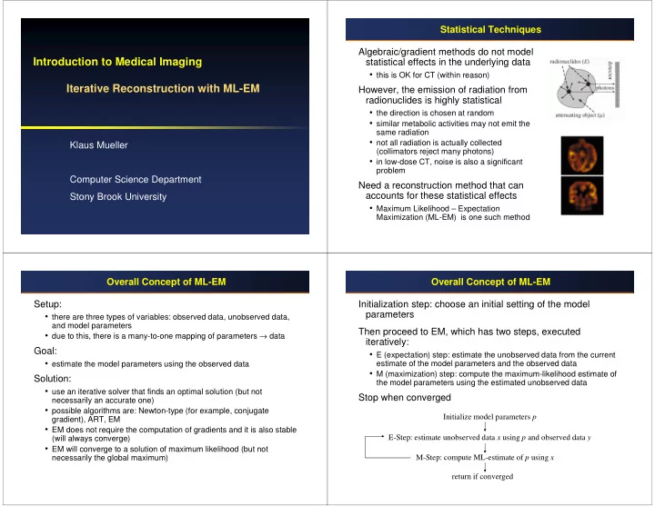
Statistical Techniques Algebraic/gradient methods do not model Introduction to Medical Imaging statistical effects in the underlying data • this is OK for CT (within reason) Iterative Reconstruction with ML-EM However, the emission of radiation from radionuclides is highly statistical • the direction is chosen at random • similar metabolic activities may not emit the same radiation • not all radiation is actually collected Klaus Mueller (collimators reject many photons) • in low-dose CT, noise is also a significant problem Computer Science Department Need a reconstruction method that can accounts for these statistical effects Stony Brook University • Maximum Likelihood – Expectation Maximization (ML-EM) is one such method Overall Concept of ML-EM Overall Concept of ML-EM Setup: Initialization step: choose an initial setting of the model parameters • there are three types of variables: observed data, unobserved data, and model parameters Then proceed to EM, which has two steps, executed • due to this, there is a many-to-one mapping of parameters → data iteratively: Goal: • E (expectation) step: estimate the unobserved data from the current • estimate the model parameters using the observed data estimate of the model parameters and the observed data • M (maximization) step: compute the maximum-likelihood estimate of Solution: the model parameters using the estimated unobserved data • use an iterative solver that finds an optimal solution (but not Stop when converged necessarily an accurate one) • possible algorithms are: Newton-type (for example, conjugate Initialize model parameters p gradient), ART, EM • EM does not require the computation of gradients and it is also stable E-Step: estimate unobserved data x using p and observed data y (will always converge) • EM will converge to a solution of maximum likelihood (but not necessarily the global maximum) M-Step: compute ML-estimate of p using x return if converged

The Poisson Distribution Relation to Functional Imaging Also called the law of rare events The observed data, y(d), are the detector readings • it is the binomial distribution of k as the number of trials n goes to infinity The unobserved data, x(b), are the photon emission activities in the pixels (the tissue) • these give rise to the detector readings • with p = λ / n • they follow a Poisson distribution The model parameters, λ( b ) , are the metabolic properties of the pixels (the tissue) λ : expected number of events (the mean) in a given time interval • these cause the emissions • they represent the expectations (means) of the resulting Poisson Some examples for Poisson-distributed events: k distribution causing the readings at the detectors • the number of phone calls at a call center per minute • the number of spelling errors a secretary makes while typing a single page • the number of soldiers killed by horse-kicks each year in each corps in the Prussian cavalry Note: to conform with the literature we shall use the terms • the number of positron emissions in a radio nucleotide in PET and SPECT (object) pixels and (detector) bins here • the number of annihilation events in PET and SPECT Relation to Functional Imaging Derivation Since there is a many-to-one mapping, many objects are The mathematical model is based on the assumption that the emissions occur according to a spatial Poisson point process in the region of interest probable to have produced the observed data (field of view) in the source. • the object reconstruction (the image ) having the highest such • for each box b there is a Poisson distributed random variable x(b), with mean probability is the maximum likelihood estimate of the original object λ( b ) , that can be generated independently: We shall use the following variables: • x [ b :1… B ]: the discretized image with B pixels (boxes) • y [ d :1… D ]: the data (the projections), D is the number of detector bins Suppose now, that an emission in the b -th box is detected in the d -th tube (tubes) with known probability The reconstruction is based on some mathematical model that p(b,d) = P ( event detected in tube d | event emitted in box b ) relates parameters, observed and unobserved data • the probability matrix p ( b,d ) is assumed to be known from the detector array geometry and other characteristics of the system (attenuation, scatter, etc) • the probability of an event in box b to be detected by the scanner is given by: D � ≤ p ( b , d ) 1 d = 1 • thus, photons do go undetected

Derivation Derivation The variables y(d) are independent and Poisson, with For any set of detector data y(d) there are many different expectation λ( d ) where: ways the photons could have been generated. • thus there is a many-to-one mapping x(b,d) to y(d) • this mapping is Poisson distributed with mean: Since the x(i) are independent Poisson variables, a linear The likelihood function is then: combination of these variables is also Poisson distributed. • the expectation of the observed data is therefore linked with the model parameters: and the log-likelihood is: λ( d ) then expresses the expectation (under the Poisson probability model for emission) to observe the given counts in the detector tubes if the true density is λ( b ). Derivation Derivation In the M-step we maximize λ [k] (b) using x [k+1] : For the E-step we compute: since • x(b,d) is Poisson with mean λ [k] ( b,d ) • is Poisson with mean • one can write, after some manipulations: Combining the E and the M steps:

Algorithm Comments There are a number of properties: 1. Start with an initial estimate λ [0] (b) satisfying x(0)(b) > 0, b=1,2,...,B • since the correction is multiplicative, all images produced are non- negative (compare the algebraic reconstruction methods) 2. If λ [k] (b) denotes the estimate of λ (b) at the k- th iteration, • the algorithm is also self-normalizing : the redistribution of the activity in the image cells which occurs after each iteration is done without define a new estimate λ [k+1] (b) by: any net increase or decrease in the total activity The EM algorithm for emission tomography can provide a physically accurate reconstruction model • it allows the direct incorporation of many physical factors, which, if not accounted for, can introduce errors in the final reconstruction. • these factors can be included in the transition matrix p(b,d): - detector response 3. If the required accuracy for the numerical convergence has - attenuation correction information been achieved, then stop - scatter modeling - positron range and angulation effects - time-of-flight information - and others Comments Comments Stopping criterion: Comparing EM to Filtered Backprojection • advantages: - less streak artifacts and noise - projection data can be irregularly spaced • stop when this residual goes to a small number, or grows again • disadvantages: • typically, noise and the edge artifacts lead to growth in the residual - much slower due to iterative scheme after reaching he optimum point - may produce streak artifacts at the edges Acceleration: • most popular is Ordered Subsets (OS) EM • here the update is done after every subset of projections • note: this method does not converge to a maximum likelihood solution, except for the case of noise-free data. Acceleration can provide faster convergence towards high- likelihood estimates, however, it does not guarantee a better image quality • various modified MLE techniques exist, which incorporate a priori information to characterize the source distribution and the data noise.