Introduction to Medical Imaging non-invasive inexpensive portable - - PowerPoint PPT Presentation

Introduction to Medical Imaging Ultrasound Imaging

Klaus Mueller Computer Science Department Stony Brook University Overview Advantages

• non-invasive
• inexpensive
• portable
• excellent temporal resolution

Disadvantages

• noisy
• low spatial resolution

Samples of clinical applications

• echo ultrasound
• cardiac
• fetal monitoring
• Doppler ultrasound
• blood flow
• ultrasound CT
• mammography

US guided biopsy Doppler effect

History Milestone applications:

• publication of The Theory of Sound (Lord Rayleigh, 1877)
• discovery of piezo-electric effect (Pierre Curie, 1880)
• enabled generation and detection of ultrasonic waves
• first practical use in World War One for detecting submarines
• followed by
• non-destructive testing of metals (airplane wings, bridges)
• seismology
• first clinical use for locating brain tumors (Karl Dussik,

Friederich Dussik, 1942)

• the first greyscale images were produced in 1950
• in real time by Siemens device in 1965
• electronic beam-steering using phased-array technology in 1968
• popular technique since mid-70s
• substantial enhancements since mid-1990

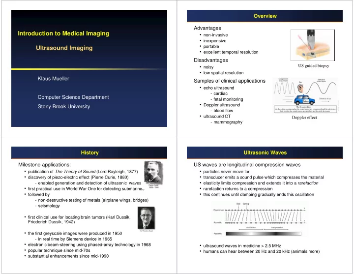
Ultrasonic Waves US waves are longitudinal compression waves

• particles never move far
• transducer emits a sound pulse which compresses the material
• elasticity limits compression and extends it into a rarefaction
• rarefaction returns to a compression
• this continues until damping gradually ends this oscillation
• ultrasound waves in medicine > 2.5 MHz
• humans can hear between 20 Hz and 20 kHz (animals more)

Generation of Ultrasonic Waves Via piezoelectric crystal

• deforms on application of electric field generates a pressure wave
• induces an electric field upon deformation  detects a pressure wave
• such a device is called transducer

Two equations

• wave equation:

∆p: acoustic pressure, ρ0: acoustic density , βs0: adiabatic compressibility

• Eikonal equation:

1/F: “slowness vector”, inversely related to acoustic velocity v

• models a surface of constant phase called the wave front
• sound rays propagate normal to the wave fronts and define the

direction of energy propagation.

Wave Propagation

2 2 2 2

1 1

s

p p c c t ρ β ∂ ∆ ∇ ∆ = = ∂

2 2 2 2 2 2 2

1 ( , , ) t t t x y z F x y z ∂ ∂ ∂ + + = ∂ ∂ ∂

Effects in Homogeneous Media Attenuation

• models the loss of energy in tissue
• f: frequency, typically n=1, z: depth,

a0: attenuation coefficient of medium,

Non-linearity

• wave equation was derived assuming that ∆p was only a tiny

disturbance of the static pressure

• however, with increasing acoustic pressure, the wave changes shape

and the assumption is violated

Diffraction

• complex interference pattern greatest

close to the source

• further away point sources add constructively

( , )

n

a f z

H f z e− =

simulation with a circular planar source

Effects in Non-Homogeneous Media (1) Reflection and refraction

• at a locally planar interface the wave’s frequency will not change, only

its speed and angle

• for c2 > c1 and θi > sin-1(c1/c2) the

reflected wave will not be in phase when is complex

• the amplitude changes as well: T+R=1, Z=ρ v

1 1 2

sin sin sin

i r t

c c c θ θ θ = =

2 2 1

cos 1 ( sin )

t i

c c θ θ = −

1 2 1 2 1 2 1

2 cos cos cos R cos cos cos cos

t t r i t i i t i i t

A Z A Z Z T A Z Z A Z Z θ θ θ θ θ θ θ − = = = = + +

Effects in Non-Homogeneous Media (2) Scattering

• if the size of the scattering object is << λ then get constructive

interference at a far-enough receiver P

• if not, then need to model scattering as many point scatterers for a

complex interference pattern small object << λ large object

Data Acquisition: A-Mode ‘A’ for Amplitude Simplest mode (no longer in use), basically:

• clap hands and listen for echo:
• time and amplitude are almost

equivalent since sound velocity is about constant in tissue

Problem: don’t know where sound bounced off from

• direction unclear
• shape of object unclear
• just get a single line

time expired speed of sound distance = 2 ⋅ pulse sent out  echo received

Data Acquisition: M-Mode ‘M’ for Motion Repeated A-mode measurement Very high sampling frequency: up to 1000 pulses per second

• useful in assessing rates and motion
• still used extensively in cardiac and fetal cardiac imaging

motion of heart wall during contraction pericardium blood heart muscle

Data Acquisition: B-Mode ‘B’ for Brightness An image is obtained by translating or tilting the transducer

fetus normal heart continuous

Image Reconstruction (1) Filtering

• remove high-frequency noise

Envelope correction

• removes the high frequencies of the RF signal

Attenuation correction

• correct for pulse attenuation at increasing depth
• use exponential decay model

Image Reconstruction (2) Log compression

• brings out the low-amplitude speckle noise
• speckle pattern can be used to distinguish

different tissue

Acquisition and Reconstruction Time Typically each line in an image corresponds to 20 cm

• velocity of sound is 1540 m/s

time for line acquisition is 267 µs

• an image with 120 lines requires then about 32 ms

can acquire images at about 30 Hz (frames/s)

• clinical scanners acquire

multiple lines simultaneously and achieve 70-80 Hz

Doppler Effect: Introduction

Doppler Effect: Fundamentals (1) Assume an acoustic source emits a pulse of N oscillation within time ∆tT

• a point scatterer Ps travels at axial velocity va:
• the locations of the wave and the scatterer are:
• the start of the wave meets Ps at:
• the end of the wave meets Ps at:
• the start of the wave meets the transducer at
• the end of the wave meets the transducer at

( ) ( )

b s a

P t ct P t d v t = = + ( ) ( )

b ib s ib ib a

d P t P t t c v = → = − ( ) ( )

T b ie s ie ie ib T a a

d c t c P t P t t t t c v c v + ∆ = → = = + ∆ − − 2

rb ib

t t = 2

re ie T

t t t = − ∆

Doppler Effect: Fundamentals (2) Received pulse (N oscillations)

• the duration of the received pulse is
• writing it as frequencies
• the Doppler frequency is then
• to hear this frequency, add it to some base frequency fb
• finally, to make the range smaller, fd may have to be scaled

Example:

• assume a scatterer moves away at 0.5 m/s, the pulse frequency is 2.5

MHz, and a base frequency of 5 kHz, then the shift is an audible 5 kHz - 1.6 kHz = 3.4 kHz 2 ( 1)

R re rb T a

c t t t t c v ∆ = − = − ∆ −

T R T R

N N f f t t = = ∆ ∆ 2 2 cos

a a D R T T T a

v v f f f f f c v c θ − − = − = ≈ +

Doppler: CW ‘CW’ for Continuous Wave Compare frequency of transmitted wave fT with frequency of received wave fR

• the Doppler frequency is then:
• Doppler can be made audible, where pitch is analog to velocity

2 cos 2

a a D R T T T a

v v f f f f f c v c θ − − = − = ≈ +

Doppler: PW (1) ‘PW’ for Pulsed Wave Does not make use of the Doppler principle

• instead, received signal is assumed to be a scaled, delayed replica of

the transmitted one ∆t is the time between transmission and reception of the pulse it depends on the distance between transducer and scatterer

• in fact, we only acquire one sample of each of the

received pulses, at tR:

• now, if the scatterer moves away at velocity va, then the distance

increases with va TPRF (TPRF: pulse repetition period)

• this increases the time ∆t (or decreases if the scatterer comes closer)

( ) sin(2 ( ))

T

s t A f t t π = − ∆ ( ) sin(2 ( ))

R T R

s t A f t t π = − ∆

Doppler: PW (2) Thus, the sampled sequence sj is:

• therefore, the greater va, the higher the frequency of the sampled

sinusoid:

• to get direction information, one must sample more than once per

pulse (twice per half oscillation) : 2 sin( 2 ( ) )

a PRF j T

v T s A f j B c π ⋅ = − ⋅ + 2 a

D T

v f f c = −

Doppler: PW (3) Color Flow Imaging: Technique Calculates the phase shift between two subsequently received pulses

• measure the phase shift by sampling two subsequent

pulses at two specific time instances tR1 and tR2

• since this can become noisy, usually the results of 3-7 such

samplings (pulses) are averaged

• divide the acquired RF line into segments (range gates) allows

velocities to be obtained at a number of depths

• acquiring along a single line gives

a M-mode type display

• acquiring along multiple lines enables

a B-mode type display red: moving toward transducer blue: moving away from transducer 2 2 ( )

a PRF T

v T f c ϕ π ⋅ ∆ =

Ultrasound Equipment

Left: Linear array transducer. Right: Phased array transducer

commercial echocardiographic scanner

Ultrasound Applications (1)

Left: Normal cranial ultrasound. Right: Fluid filled cerebral cavities on both sides as a result of an intraventricular haemorrhage

Ultrasound Applications (2)

Left: normal lung, Right: pleural effusion

Ultrasound Applications (3)

Left: normal liver Right: liver with cyst

Ultrasound Applications (4)

Left: prostate showing a hypoechoic lesion suspicious for cancer Right: with biopsy needle

Ultrasound Applications (5)

Atrial septal defect (ASD)

Ultrasound Applications (6)

Doppler color flow image of a patient with mitral regurgitation in the left

• atrium. The bright green color corresponds to high velocities in mixed

directions, due to very turbulent flow leaking through a small hole in the mitral valve.