Information Visualization networks without networks, couldn't - - PowerPoint PPT Presentation

information visualization
SMART_READER_LITE
LIVE PREVIEW

Information Visualization networks without networks, couldn't - - PowerPoint PPT Presentation

Network data Applications of networks Information Visualization networks without networks, couldn't have any of these: Dataset Types model relationships Networks & Trees 1/2 between things Tables Networks Fields (Continuous)


slide-1
SLIDE 1

https://www.cs.ubc.ca/~tmm/courses/436V-20

Information Visualization Networks & Trees 1/2

Tamara Munzner Department of Computer Science University of British Columbia

Lect 14/15, Feb 27 & Mar 3 2020

Network data

  • networks

–model relationships between things

  • aka graphs

–two kinds of items, 
 both can have attributes

  • nodes
  • links
  • tree

–special case –no cycles

  • one parent per node

2

Dataset Types Tables

Attributes (columns) Items (rows) Cell containing value

Networks

Link Node (item)

Trees

Fields (Continuous)

Attributes (columns) Value in cell

Cell

Multidimensional Table

Value in cell

Grid of positions

Networks

3

Applications of networks

  • without networks, couldn't have any of these:

4

Applications of networks: biological networks

  • interactions between genes, proteins, and chemical products
  • the brain: connections between neurons
  • your ancestry: the relations between you and your family
  • phylogeny: the evolutionary relationships of life

5

Phylogeny: the evolutionary relationships of life

[Beyer 2014]

6

Exercise: Friend networks, two ways

  • Imagine a network of friends

–you want to visualize if and how often the friends have met each other –for each friend you have age, gender, and origin info

  • Create two different sketches that visualize this friendship relation
  • In Socrative quiz, click on true when done 


[~5 min]

7

Network tasks: topology-based

  • topological structure of network

–path following

  • path is route along links

– hops from one node to another

  • path length is number of links along route

– shortest path connects nodes i & j with smallest #

  • f hops
  • topology vs geometry

–topological hops different from geometric distance given specific layout

  • topology does not depend on layout
  • geometry does

8

Network tasks: topology-based

  • topological structure of network

–node importance metrics

  • node degree: attribute on nodes

– number of links connected to a node – local measure of importance – average degree, degree distribution

9

Degree distribution

  • real network

–power law distributions are common

10

Protein interaction network, Barabasi

Network tasks: topology-based

  • topological structure of network

–node importance metrics

  • betweenness centrality: attribute on nodes

– how many shortest paths pass through a node – global measure of importance – good measure for overall relevance of node in network

11

Centrality measures: Degree vs betweenness centrality

12

Network tasks: attribute-based vs topology-based

  • topology based tasks

–find paths –find (topological) neighbors –compare centrality/importance measures –identify clusters / communities

  • attribute based tasks (similar to table data)

–find extreme values, ...

  • combination tasks - incorporating both
  • example: locate - find single or multiple nodes/links with a given property

–topology: find all adjacent nodes of given node –attributes: find edges with maximum edge weight

13

Three kinds of network visual encodings

14

Node–Link Diagrams Enclosure Adjacency Matrix

TREES NETWORKS

Connection Marks

TREES NETWORKS

Derived Table

TREES NETWORKS

Containment Marks

Node-link diagrams

  • nodes: point marks
  • links: line marks

–straight lines or arcs –connections between nodes

  • intuitive & familiar

–most common –many, many variants

15

Node–Link Diagrams

TREES NETWORKS

Connection Marks

A C B D E

Free Styled Fixed

HJ Schulz 2006

Exercise

  • sketch an aesthetically pleasing node-link diagram of this network

–there are five nodes: A,B,C,D,E –each row in the table describes an edge A B C D C B A D A C B D D E A E

  • Socrative quiz: pick true when done [~5 min]

16

slide-2
SLIDE 2

Criteria for good node-link layouts

  • minimize

–edge crossings –distances between topological neighbor nodes –total drawing area –edge bends –edge length disparities (sometimes)

  • maximize

–angular distance between different edges –aspect ratio disparities

  • emphasize symmetry

–similar graph structures should look similar in layout

17

Criteria conflict

  • most criteria NP-hard individually
  • many criteria directly conflict with each other

18

Minimum number


  • f edge crossings


 vs.
 
 Uniform edge length Space utilization
 
 vs.
 
 Symmetry

Schulz 2004

Optimization-based layouts

  • formulate layout problem as optimization problem
  • convert criteria into weighted cost function

–F(layout) = a*[crossing counts] + b*[drawing space used]+...

  • use known optimization techniques to find layout at minimal cost

–energy-based physics models –force-directed placement –spring embedders

19

Force-directed placement

  • physics model

–links = springs pull together –nodes = magnets repulse apart

  • algorithm

–place vertices in random locations –while not equilibrium

  • calculate force on vertex

– sum of » pairwise repulsion of all nodes » attraction between connected nodes

  • move vertex by c * vertex_force

20

  • uts

magnets

Spring Coil
 (pulling nodes together) Expander 
 (pushing nodes apart)

http://mbostock.github.com/d3/ex/force.html

Force-directed placement properties

  • strengths

–reasonable layout for small, sparse graphs –clusters typically visible –edge length uniformity

  • weaknesses

–nondeterministic –computationally expensive: O(n^3) for n nodes

  • each step is n^2, takes ~n cycles to reach equilibrium

–naive FD doesn't scale well beyond 1K nodes –iterative progress: engaging but distracting

21

https://bl.ocks.org/steveharoz/8c3e2524079a8c440df60c1ab72b5d03

Idiom: force-directed placement

  • visual encoding

– link connection marks, node point marks

  • considerations

– spatial position: no meaning directly encoded

  • left free to minimize crossings

– proximity semantics?

  • sometimes meaningful
  • sometimes arbitrary, artifact of layout algorithm
  • tension with length

– long edges more visually salient than short

  • tasks

– explore topology; locate paths, clusters

  • scalability

– node/edge density E < 4N

22

http://mbostock.github.com/d3/ex/force.html

Multilevel approaches

  • derive cluster hierarchy of metanodes on top of original graph nodes

23

[Schulz 2004] real vertex virtual vertex internal spring external spring virtual spring Metanode A Metanode B Metanode C

Idiom: sfdp (multi-level force-directed placement)

  • data

–original: network –derived: cluster hierarchy atop it

  • considerations

–better algorithm for same encoding technique

  • same: fundamental use of space
  • hierarchy used for algorithm speed/quality but

not shown explicitly

  • scalability

–nodes, edges: 1K-10K –hairball problem eventually hits

24

[Efficient and high quality force-directed graph drawing. Hu. The Mathematica Journal 10:37–71, 2005.]

http://www.research.att.com/yifanhu/GALLERY/GRAPHS/index1.html

Restricted layouts: Circular, arc

  • lay out nodes around circle or along line

– circular layouts – arc diagrams

  • node ordering crucial to avoid excessive clutter


from edge crossings

– barycentric ordering before & after – derived attribute: global computation

25

http://profs.etsmtl.ca/mmcguffin/research/2012-mcguffin-simpleNetVis/mcguffin-2012-simpleNetVis.pdf

Edge clutter reduction: hierarchical edge bundling

26

[Hierarchical Edge Bundles: Visualization of Adjacency Relations in Hierarchical Data. Danny Holten. TVCG 12(5):741-748 2006]

Hierarchical edge bundling

27

[Hierarchical Edge Bundles: Visualization of Adjacency Relations in Hierarchical Data. Danny Holten. TVCG 12(5):741-748 2006] Bundling Strength

Bundle strength

28

http://mbostock.github.io/d3/talk/20111116/bundle.html

Fixed layouts: Geographic

  • lay out network nodes using given/fixed

spatial data

–route edges accordingly –edge bundling also applicable

29

https://www.facebook.com/notes/facebook-engineering/visualizing-friendships/469716398919

Adjacency matrix representations

  • derive adjacency matrix from network

30

A C B D E A B C D E A B C D E

Adjacency matrix examples

31

:

HJ Schulz 2007

Node order is crucial: Reordering

32

https://bost.ocks.org/mike/miserables/

slide-3
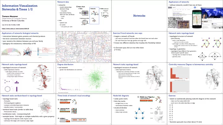
SLIDE 3

Adjacency matrix

  • ˜

33

Well suited for 
 Not suited for 


good for topology tasks
 related to neighborhoods (node 1-hop neighbors) bad for topology tasks
 related to paths

Structures visible in both

34

http://www.michaelmcguffin.com/courses/vis/patternsInAdjacencyMatrix.png

Idiom: adjacency matrix view

  • data: network

–transform into same data/encoding as heatmap

  • derived data: table from network

–1 quant attrib

  • weighted edge between nodes

–2 categ attribs: node list x 2

  • visual encoding

–cell shows presence/absence of edge

  • scalability

–1K nodes, 1M edges

35

[NodeTrix: a Hybrid Visualization of Social Networks. Henry, Fekete, and McGuffin. IEEE TVCG (Proc. InfoVis) 13(6):1302-1309, 2007.] [Points of view: Networks. Gehlenborg and

  • Wong. Nature Methods 9:115.]

Node-link vs. matrix comparison

  • node-link diagram strengths

–topology understanding, path tracing –intuitive, flexible, no training needed

  • adjacency matrix strengths

–focus on edges rather than nodes –layout straightforward (reordering needed) –predictability, scalability –some topology tasks trainable

  • empirical study

–node-link best for small networks –matrix best for large networks

  • if tasks don’t involve path tracing!

36

[On the readability of graphs using node-link and matrix-based representations: a controlled experiment and statistical analysis. Ghoniem, Fekete, and Castagliola. Information Visualization 4:2 (2005), 114–135.] http://www.michaelmcguffin.com/courses/vis/patternsInAdjacencyMatrix.png

Idiom: NodeTrix

  • hybrid nodelink/matrix
  • capture strengths of both

37

NodeTrix
 [Henry et al. 2007]

Trees

38

Tree exercise

  • socrative: true when done with both

39

Here is part of a directory structure used for the material for this class and the relative file size. datavis-17/ lectures/ Intro.key (110 MB) perception/ Perception.key (113 MB) Blindness.mov (15MB) Data.key (12 MB) Graphs.key (180 MB) exams/ Exam1-solution.doc (5MB) Exam1.doc (1MB) exercise/ Graph.doc (3MB) Graph-video.doc (210MB)

Sketch two different visualizations that show both, the directory structure and the size of the directories and the contained files.

Node-link trees

  • Reingold-Tilford

–tidy drawings of trees

  • exploit parent/child structure

–allocate space: compact w/o

  • verlap
  • rectilinear and radial variants

–nice algorithm writeup

40

http://bl.ocks.org/mbostock/4339184 http://bl.ocks.org/mbostock/4063550

http://billmill.org/pymag-trees/

Idiom: radial node-link tree

  • data

–tree

  • encoding

–link connection marks –point node marks –radial axis orientation

  • angular proximity: siblings
  • distance from center: depth in tree
  • tasks

–understanding topology, following paths

  • scalability

–1K - 10K nodes

41

http://mbostock.github.com/d3/ex/tree.html

!"#$ " % " & ' ( ) * + *&,+($#

  • ..&/0$#"()1$2&,+($#

2 / , % ) ( ' 3 ( # , * ( , # $ 4)$#"#*5)*"&2&,+($# 6$#.$78.$ . # " 9 5 :$(;$$%%$++2$%(#"&)(' < ) % = > ) + ( " % * $ 6 " ? @ & / ; 6 ) % 2 , ( 35/#($+(A"(5+ 39"%%)%.B#$$ / 9 ( ) ) C " ( ) / %

  • +

9 $ * ( D " ( ) / : " % = $ # "%)0"($ 7"+)%. @,%*()/%3$E,$%*$ ) % ( $ # 9 / & " ( $

  • ##"'F%($#9/&"(/#

2/&/#F%($#9/&"(/# > " ( $ F % ( $ # 9 / & " ( / # F % ( $ # 9 / & " ( / # 6 " ( # ) ? F % ( $ # 9 / & " ( / # G , H $ # F % ( $ # 9 / & " ( / # IHJ$*(F%($#9/&"(/# A/)%(F%($#9/&"(/# D$*("%.&$F%($#9/&"(/# F3*5$8,&"H&$ A"#"&&$& A",+$ 3 * 5 $ 8 , & $ # 3$E,$%*$ B # " % + ) ( ) / % B#"%+)()/%$# B # " % + ) ( ) / % 7 1 $ % ( B;$$% 8 " ( " */%1$#($#+ 2 / % 1 $ # ( $ # + >$&)0)($8B$?(2/%1$#($# K#"956<2/%1$#($# F>"("2/%1$#($# L 3 I G 2 / % 1 $ # ( $ # >"("@)$&8 >"("3*5$0" > " ( " 3 $ ( >"("3/,#*$ >"("B"H&$ >"("M()& 8)+9&"' >)#('39#)($ <)%$39#)($ D $ * ( 3 9 # ) ( $ B $ ? ( 3 9 # ) ( $ ! $ ? @ & " # $ N ) + 95'+)*+ >#".@/#*$ K#"1)('@/#*$ F@/#*$ G:/8'@/#*$ A " # ( ) * & $ 3)0,&"()/% 39#)%. 39#)%.@/#*$ E , $ # '

  • ..#$."($7?9#$++)/%
  • %8
  • #)(50$()*
  • 1$#".$

:)%"#'7?9#$++)/% 2 / 9 " # ) + / % 2/09/+)($7?9#$++)/% 2/,%( >"($M()& > ) + ( ) % * ( 7?9#$++)/% 7 ? 9 # $ + + ) / % F ( $ # " ( / # @% FO F +

  • <)($#"&

6 " ( * 5 6"?)0,0 $ ( 5 / 8 + "88 "%8 " 1 $ # " . $ */,%( 8)+()%*( 8 ) 1 $E O% .( .($ )OO )+" &( & ( $ 0"? 0)% / 8 , & %$E %/( /# / # 8 $ # H ' # " % . $ +$&$*( +(88$1 +,H +,0 , 9 8 " ( $ 1"#)"%*$ ;5$#$ ? / # P 6 ) % ) , G/( I# Q , $ # ' D"%.$ 3(#)%.M()& 3,0 N"#)"H&$ N"#)"%*$ R / # + * " & $ F3*"&$6"9 < ) % $ " # 3 * " & $ < / . 3 * " & $ I#8)%"&3*"&$ Q,"%()&$3*"&$ Q , " % ( ) ( " ( ) 1 $ 3 * " & $ D//(3*"&$ 3 * " & $ 3 * " & $ B ' 9 $ B)0$3*"&$ , ( ) &

  • ##"'+

2 / & / # + >"($+ >)+9&"'+ @)&($# K$/0$(#' 5$"9 @ ) H / % " * * ) 4 $ " 9 4$"9G/8$ F 7 1 " & , " H & $ FA#$8)*"($ F N " & , $ A # / ? ' " ( 5 >$%+$6"(#)? F 6 " ( # ) ? 39"#+$6"(#)? 6"(5+ I#)$%("()/% 9"&$(($ 2/&/#A"&$(($ A"&$(($ 3 5 " 9 $ A " & $ ( ( $ 3 ) C $ A " & $ ( ( $ A # / 9 $ # ( ' 35"9$+ 3/#( 3("(+ 3(#)%.+ 1 ) + "?)+

  • ?

$ +

  • ?)+
  • ?)+K#)8<)%$
  • ?)+<"H$&

2"#($+)"%-?$+ */%(#/&+

  • %*5/#2/%(#/&

2 & ) * = 2 / % ( # / & 2/%(#/& 2/%(#/&<)+( > # " . 2 / % ( # / & 7?9"%82/%(#/& 4/1$#2/%(#/& F2/%(#/& A"%S//02/%(#/& 3$&$*()/%2/%(#/& B//&()92/%(#/& 8 " ( " >"(" >"("<)+( >"("39#)($ 78.$39#)($ G / 8 $ 3 9 # ) ( $ #$%8$#

  • ##/;B'9$

78.$D$%8$#$# FD$%8$#$# 35"9$D$%8$#$# 3*"&$:)%8)%. B#$$ B # $ $ : , ) & 8 $ # $1$%(+ >"("71$%( 3 $ & $ * ( ) / % 7 1 $ % ( B//&()971$%( N ) + , " & ) C " ( ) / % 7 1 $ % ( & $ . $ % 8 <$.$%8 < $ . $ % 8 F ( $ <$.$%8D"%.$ / 9 $ # " ( / # 8 ) + ( / # ( ) / % :)O/*"&>)+(/#()/% > ) + ( / # ( ) / % @)+5$'$>)+(/#()/% $%*/8$# 2 / & / # 7 % * / 8 $ # 7%*/8$# A#/9$#('7%*/8$# 35"9$7%*/8$# 3 ) C $ 7 % * / 8 $ # T&($# @)+5$'$B#$$@)&($# K#"95>)+("%*$@)&($# N)+)H)&)('@)&($# FI9$#"(/# &"H$& <"H$&$# D"8)"&<"H$&$# 3("*=$8-#$"<"H$&$# &"'/,(

  • ?)+<"'/,(

:,%8&$878.$D/,($# 2)#*&$<"'/,( 2)#*&$A"*=)%.<"'/,( >$%8#/.#"0<"'/,( @ / # * $ > ) # $ * ( $ 8 < " ' / , ( F * ) * & $ B # $ $ < " ' / , ( F%8$%($8B#$$<"'/,( <"'/,( G/8$<)%=B#$$<"'/,( A)$<"'/,( D"8)"&B#$$<"'/,( D " % 8 / < " ' / , ( 3 ( " * = $ 8

  • #

$ " < " ' / , ( B # $ $ 6 " 9 < " ' / , ( I9$#"(/# I9$#"(/#<)+( I9$#"(/#3$E,$%*$ I 9 $ # " ( / # 3 ; ) ( * 5 3/#(I9$#"(/# N)+,"&)C"()/%

Containment (implicit) layouts

42

Treemap Sunburst Icicle Plot

Idiom: treemap

  • data

–tree –1 quant attrib at leaf nodes

  • encoding

–area containment marks for hierarchical structure –rectilinear orientation –size encodes quant attrib

  • tasks

–query attribute at leaf nodes

  • scalability

–1M leaf nodes

43

http://tulip.labri.fr/Documentation/3_7/userHandbook/html/ch06.html

Treemap software: disk space

44

Mac: GrandPerspective Windows: Sequoia View Containment: Approaches compared

45

Only Leaves Visible Inner Nodes and Leaves Visible

Link marks: Connection and containment

  • marks as links (vs. nodes)

–common case in network drawing –1D case: connection

  • ex: all node-link diagrams
  • emphasizes topology, path tracing
  • networks and trees

–2D case: containment

  • ex: all treemap variants
  • emphasizes attribute values at leaves (size coding)
  • only trees

46

Node–Link Diagram Treemap

[Elastic Hierarchies: Combining Treemaps and Node-Link

  • Diagrams. Dong, McGuffin, and Chignell. Proc. InfoVis

2005, p. 57-64.]

Containment Connection

Tree drawing idioms comparison

  • data shown

– link relationships – tree depth – sibling order

  • design choices

– connection vs containment link marks – rectilinear vs radial layout – spatial position channels

  • considerations

– redundant? arbitrary? – information density?

  • avoid wasting space
  • consider where to fit labels!

47

[Quantifying the Space-Efficiency of 2D Graphical Representations of

  • Trees. McGuffin and Robert. Information

Visualization 9:2 (2010), 115–140.]

treevis.net: many, many options

48

https://treevis.net/

slide-4
SLIDE 4

Idiom: GrouseFlocks

49

  • data: compound graphs

–network –cluster hierarchy atop it

  • derived or interactively chosen
  • visual encoding

–connection marks for network links –containment marks for hierarchy –point marks for nodes

  • dynamic interaction

–select individual metanodes in hierarchy to expand/ contract

[GrouseFlocks: Steerable Exploration of Graph Hierarchy Space. Archambault, Munzner, and Auber. IEEE TVCG 14(4): 900-913, 2008.] Graph Hierarchy 1

Hierarchical edge bundling: treemap vs radial

50

Credits

  • Visualization Analysis and Design (Ch 9)
  • Alex Lex & Miriah Meyer, http://dataviscourse.net/

51