IE1206 Embedded Electronics Le1 Le2 PIC-block Documentation, - - PowerPoint PPT Presentation

IE1206 Embedded Electronics

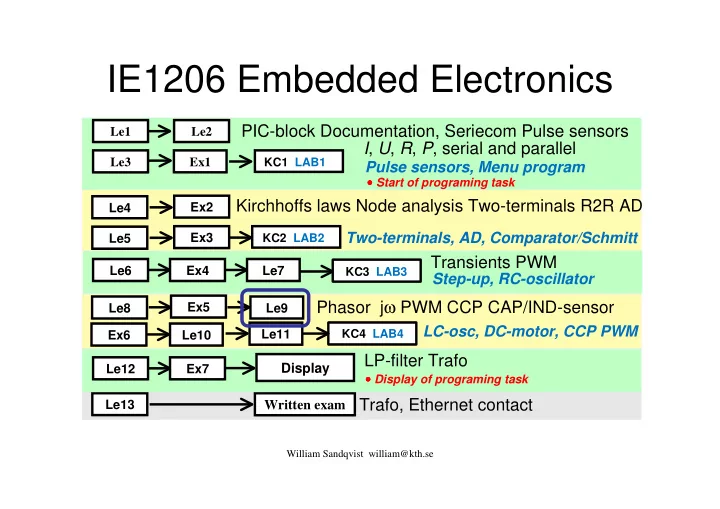
Transients PWM Phasor jω PWM CCP CAP/IND-sensor

Le1 Le3 Le6 Le8 Le2 Ex1 Le9 Ex4 Le7

Written exam

William Sandqvist william@kth.se

PIC-block Documentation, Seriecom Pulse sensors I, U, R, P, serial and parallel

Ex2 Ex5

Kirchhoffs laws Node analysis Two-terminals R2R AD Trafo, Ethernet contact

Le13

Pulse sensors, Menu program

Le4

KC1 LAB1 KC3 LAB3 KC4 LAB4

Ex3 Le5

KC2 LAB2

Two-terminals, AD, Comparator/Schmitt Step-up, RC-oscillator

Le10 Ex6

LC-osc, DC-motor, CCP PWM

LP-filter Trafo

Le12 Ex7

Display

Le11

• Start of programing task
• Display of programing task

William Sandqvist william@kth.se

R L C

An impedance which contain inductors and capacitors have, depending on the frequency, either inductive character IND, or capacitive character CAP. An important special case occurs at the frequency where capacitances and inductances are equally strong, and their effects cancel each other out. The impedance becomes purely resisistiv. The phenomenon is called the resonance and the frequency on which this occurs is the resonant frequency.

CAP

William Sandqvist william@kth.se

Reactance frequency dependency

f C X L X

C L

π ω ω ω 2 1 = ⋅ = ⋅ = ] [Ω

L

X ] [Ω

L

X ] Hz [ f ] Hz [ f

William Sandqvist william@kth.se

R L C impedances

f C X L X

C L

π ω ω ω 2 1 = ⋅ = ⋅ = ] [Ω X ] Hz [ f

• At a certain frequence XL and XC has the same amount.

William Sandqvist william@kth.se

William Sandqvist william@kth.se

How big is U ? (13.1)

The three volt meters show the same, 1V, how much is the alternating supply voltage U ? (Warning, teaser)

William Sandqvist william@kth.se

How big is U ? (13.1)

The three volt meters show the same, 1V, how much is the alternating supply voltage U ? (Warning, teaser)

William Sandqvist william@kth.se

How big is U ? (13.1)

C L R X X R ω ω 1

C L

= = = =

Since volt meters show the "same" and the current I is common:

The three volt meters show the same, 1V, how much is the alternating supply voltage U ? (Warning, teaser)

William Sandqvist william@kth.se

If |XL|=|XC|=2R ?

Suppose the AC voltage U still 1 V, but the reactances are twice as big. What will the voltmeters show?

R C L ⋅ = = 2 1 ω ω

William Sandqvist william@kth.se

If |XL|=|XC|=2R ?

R C L ⋅ = = 2 1 ω ω

Suppose the AC voltage U still 1 V, but the reactances are twice as big. What will the voltmeters show?

William Sandqvist william@kth.se

If |XL|=|XC|=2R ?

R C L ⋅ = = 2 1 ω ω

At resonance, the voltage over the reactances can be many times higher than the AC supply voltage.

Suppose the AC voltage U still 1 V, but the reactances are twice as big. What will the voltmeters show?

William Sandqvist william@kth.se

Tesla coil

Many builds "Tesla" coils to gain some excitement in life…

William Sandqvist william@kth.se

Inductor quality factor Q

IN UT L

U Q U r L r X Q ⋅ ≈

• =

= ω

Usually it is the internal resistance

• f the coil which is the resistor in

the RLC circuit. The higher the coil AC resistance ωL is in relation to the DC resistance r, the larger the voltage across the coil at a resonance get. This ratio is called the coil quality factor Q. ( or Q-factor ).

William Sandqvist william@kth.se

Series resonance

• −

+ ⋅ =

• +

+ ⋅ = ) 1 ( j j 1 j C L r I C L r I U ω ω ω ω

r

William Sandqvist william@kth.se

Series resonance

• −

+ ⋅ =

• +

+ ⋅ = ) 1 ( j j 1 j C L r I C L r I U ω ω ω ω

The Impedance is real when the imaginary part is ”0”. This will happen at angular frequency ω0 ( frequency f0 ).

=0 r

William Sandqvist william@kth.se

Series resonance

• −

+ ⋅ =

• +

+ ⋅ = ) 1 ( j j 1 j C L r I C L r I U ω ω ω ω

The Impedance is real when the imaginary part is ”0”. This will happen at angular frequency ω0 (frequency f0). =0

[ ]

LC f LC C L Z π ω ω ω 2 1 1 1 Im = =

• =

− =

r

William Sandqvist william@kth.se

Series resonance phasor diagram

• −

+ ⋅ = ) 1 ( j C L r I U ω ω

r

William Sandqvist william@kth.se

Series resonance phasor diagram

• −

+ ⋅ = ) 1 ( j C L r I U ω ω

r

William Sandqvist william@kth.se

Series resonance phasor diagram

• −

+ ⋅ = ) 1 ( j C L r I U ω ω

r

William Sandqvist william@kth.se

Series resonance circuit Q

• −

+ = = = ) ( j 1 1

max

ω ω ω ω ω ω Q I I r L Q LC

It is the resistance of the resonant circuit, usually coil internal resistance, which determines how pronounced resonance phenomenon becomes. It is customary to "normalize" the relationship between the different variables by introducing the resonance angular frequency ω ω ω ω0 together with the peak current Imax in the function I(ω) with parameter Q :

Normalized chart of the series resonant

• circuit. A high Q

corresponds to a narrow resonance peak.

r

William Sandqvist william@kth.se

Bandwidth BW

At two different angular frequencies becomes imaginary Im and real part Re in the denominator equal. I is then Imax/√2 (≈71%). The Bandwidth BW=∆ω is the distans between those two angular frequencies.

• −

+ = ) ( j 1

max

ω ω ω ω Q I I

Re = Im

[ ] ( )

• +

+ ± = ⋅ = = − = ∆ = 1 2 1 2 1 , rad/s

2 1 2 1 2 2 1 2

Q Q Q BW ω ω ω ω ω ω ω ω ω ω

The equations give :

William Sandqvist william@kth.se

• More convenient formulas

Q f f Q r L f Q LC f 1 1 2 2 1 = ∆

• =

∆ = = ω ω π π 2 ,

1 2

f f f f ∆ ± ≈

If Q is high, no significant error is done if the bandwidth is divided equally on both sides of f0.

William Sandqvist william@kth.se

William Sandqvist william@kth.se

Example, series resonance circuit

C = 25 nF f0 = 100 kHz BW = ∆f = 12,5 kHz Q = ? L = ? r = ?

r =?

% 71

f

William Sandqvist william@kth.se

Example, series resonance circuit

8 5 , 12 100 = = ∆ = f f Q

r =?

C = 25 nF f0 = 100 kHz BW = ∆f = 12,5 kHz Q = ? L = ? r = ?

% 71

f

William Sandqvist william@kth.se

Example, series resonance circuit

8 5 , 12 100 = = ∆ = f f Q mH 1 , 10 25 ) 10 100 2 ( 1 ) 2 ( 1 2 1

9 2 3 2

= ⋅ ⋅ ⋅ ⋅ = =

• =

−

π π π C f L LC f

r =?

C = 25 nF f0 = 100 kHz BW = ∆f = 12,5 kHz Q = ? L = ? r = ?

% 71

f

William Sandqvist william@kth.se

Example, series resonance circuit

8 5 , 12 100 = = ∆ = f f Q mH 1 , 10 25 ) 10 100 2 ( 1 ) 2 ( 1 2 1

9 2 3 2

= ⋅ ⋅ ⋅ ⋅ = =

• =

−

π π π C f L LC f Ω ≈ ⋅ ⋅ ⋅ ⋅ = ⋅ =

• ⋅

= =

−

8 8 10 1 , 10 100 2 2 2

3 3

π π π Q L f r r L f r X Q

L

r =?

C = 25 nF f0 = 100 kHz BW = ∆f = 12,5 kHz Q = ? L = ? r = ?

% 71

f

William Sandqvist william@kth.se

William Sandqvist william@kth.se

How big is I ? (13.2)

The three ammeters show the same, 1A, how much is the AC supply current I ? ( Warning, teaser )

William Sandqvist william@kth.se

How big is I ? (13.2)

The three ammeters show the same, 1A, how much is the AC supply current I ? ( Warning, teaser )

William Sandqvist william@kth.se

How big is I ? (13.2)

IL and IC becomes a circulating current decoupled from IR. IL, IC can be many times bigger than the supply current I = IR. This is parallel resonance. The three ammeters show the same, 1A, how much is the AC supply current I ? ( Warning, teaser )

William Sandqvist william@kth.se

Ideal parallel resonance circuit

) 1 ( j 1 1 j j 1 1 1 || || L C R C L R C L R Z ω ω ω ω − + = + + = = =0

The resonance frequency has exactly the same expression as for the series resonant circuit, but otherwise the circuit has reverse character, IND at low frequencies and CAP at high. At resonance, the impedance is real = R.

LC f π 2 1

0 =

William Sandqvist william@kth.se

Ideal parallel resonance circuit

) 1 ( j 1 1 j j 1 1 1 || || L C R C L R C L R Z ω ω ω ω − + = + + = = =0

LC f π 2 1

0 =

Actual parallel resonant circuit

Actual parallel resonant circuits has a series resistance inside the coil. The calculations become more complecated and the resonance frequency will also differ slightly from our formula. The resonance frequency has exactly the same expression as for the series resonant circuit, but otherwise the circuit has reverse character, IND at low frequencies and CAP at high. At resonance, the impedance is real = R.

William Sandqvist william@kth.se

William Sandqvist william@kth.se

Example, actual circuit (13.3)

• +

− + + ⋅ = =

• +

− + ⋅ = − − ⋅ + + = + = ) ) ( ( j ) ( ) ( j j ) j ( ) j ( j j 1

2 2 2 2 2 2 LR C

L r L C L r r U L r L r C U L r L r L r U C U I I I ω ω ω ω ω ω ω ω ω ω ω =0

William Sandqvist william@kth.se

Example, actual circuit (13.3)

• +

− + + ⋅ = =

• +

− + ⋅ = − − ⋅ + + = + = ) ) ( ( j ) ( ) ( j j ) j ( ) j ( j j 1

2 2 2 2 2 2 LR C

L r L C L r r U L r L r C U L r L r L r U C U I I I ω ω ω ω ω ω ω ω ω ω ω =0

• −

=

• =

− =

• +

=

2 2 2 2 2 2 2

1 2 1 2 1 ) ( L r LC f f L r LC L r L C π π ω ω ω ω ω

William Sandqvist william@kth.se

William Sandqvist william@kth.se

Metal Detector

2 2

1 1 2 r f LC L π

• =

−

• Any "losses" (even

eddy-current losses in all kinds of metals) are summarized by the symbol r ! Eddy current losses The parallel resonant frequency is affected by the coil losses. That’s how hidden treasures are found! Iron objects affects the magnetic field and thus also L !

William Sandqvist william@kth.se

William Sandqvist william@kth.se

Series or parallel resistor

In manual computation for simplicity one usually uses the formulas of the ideal resonant circuit. At high Q and close to the resonance frequency f0 the deviations becomes insignificant. At Q >10 are the two circuits "interchangeable".

S 2 P P S

r Q R L R r L Q ⋅ =

• =

= ω ω

(applies approximately for Q >10 ) Alternative definition of Q with RP

LC 1

0 ≈

ω

William Sandqvist william@kth.se

Example, parallel circuit

Parallel circuit. C = 25 nF f0 = 100 kHz BW = 1250 Hz L = ? r = ?

William Sandqvist william@kth.se

Example, parallel circuit

80 1250 10 100

3

= ⋅ = ∆ = f f Q

Parallel circuit. C = 25 nF f0 = 100 kHz BW = 1250 Hz L = ? r = ?

William Sandqvist william@kth.se

Example, parallel circuit

80 1250 10 100

3

= ⋅ = ∆ = f f Q

80 > 10 justifying counting with the ideal model. Parallel circuit. C = 25 nF f0 = 100 kHz BW = 1250 Hz L = ? r = ?

William Sandqvist william@kth.se

Example, parallel circuit

80 1250 10 100

3

= ⋅ = ∆ = f f Q mH 1 , 10 25 ) 10 100 2 ( 1 ) 2 ( 1 2 1

9 2 3 2

= ⋅ ⋅ ⋅ ⋅ = =

• =

−

π π π C f L LC f

80 > 10 justifying counting with the ideal model. Parallel circuit. C = 25 nF f0 = 100 kHz BW = 1250 Hz L = ? r = ?

William Sandqvist william@kth.se

Example, parallel circuit

80 1250 10 100

3

= ⋅ = ∆ = f f Q mH 1 , 10 25 ) 10 100 2 ( 1 ) 2 ( 1 2 1

9 2 3 2

= ⋅ ⋅ ⋅ ⋅ = =

• =

−

π π π C f L LC f Ω ≈ ⋅ ⋅ ⋅ ⋅ ⋅ = ⋅ ⋅ =

• ⋅

= =

−

5027 80 10 1 , 10 100 2 2 2

3 3 P P L P

π π π Q L f R L f R X R Q

80 > 10 justifying counting with the ideal model. Parallel circuit. C = 25 nF f0 = 100 kHz BW = 1250 Hz L = ? r = ?

William Sandqvist william@kth.se

Example, parallel circuit

80 1250 10 100

3

= ⋅ = ∆ = f f Q mH 1 , 10 25 ) 10 100 2 ( 1 ) 2 ( 1 2 1

9 2 3 2

= ⋅ ⋅ ⋅ ⋅ = =

• =

−

π π π C f L LC f Ω ≈ ⋅ ⋅ ⋅ ⋅ ⋅ = ⋅ ⋅ =

• ⋅

= =

−

5027 80 10 1 , 10 100 2 2 2

3 3 P P L P

π π π Q L f R L f R X R Q

80 > 10 justifying counting with the ideal model.

Ω ≈ = = 8 , 5027 80 1 1

2 P 2 S

R Q r

Answer with a series resistor! Parallel circuit. C = 25 nF f0 = 100 kHz BW = 1250 Hz L = ? r = ?

William Sandqvist william@kth.se

Example, parallel circuit

80 1250 10 100

3

= ⋅ = ∆ = f f Q mH 1 , 10 25 ) 10 100 2 ( 1 ) 2 ( 1 2 1

9 2 3 2

= ⋅ ⋅ ⋅ ⋅ = =

• =

−

π π π C f L LC f Ω ≈ ⋅ ⋅ ⋅ ⋅ ⋅ = ⋅ ⋅ =

• ⋅

= =

−

5027 80 10 1 , 10 100 2 2 2

3 3 P P L P

π π π Q L f R L f R X R Q

80 > 10 justifying counting with the ideal model.

Ω ≈ = = 8 , 5027 80 1 1

2 P 2 S

R Q r

Sanswer with a series resistor!

2 2

1 1 2 r f LC L π

• =

−

• Luckily we did not have

to use this formula to calculate the L Parallel circuit. C = 25 nF f0 = 100 kHz BW = 1250 Hz L = ? r = ?

William Sandqvist william@kth.se

The inductive sensor is a rugged sensor type available in many types.

William Sandqvist william@kth.se

Cyclists who request green?

Inductive sensor for bicycle Sorry! The Sensor does not work for all bicycles?

William Sandqvist william@kth.se

William Sandqvist william@kth.se