Filters and Bode magnitude plots ( corrected version ) ENGR 40M - - PDF document

SLIDE 1

Filters and Bode magnitude plots (corrected version)

ENGR 40M lecture notes — August 4, 2017 Chuan-Zheng Lee, Stanford University

The decibel

Recall that the gain of a circuit is the ratio Vout

Vin . We often express (the magnitude of) gains on a logarithmic

scale, using a unit called decibels (dB). The gain in decibels is defined as gain in dB = 20 log10

• Vout

Vin

• .

Expressing gains in decibels allows us to see a much bigger range with reasonable numbers. For example, it’s hard to distinguish between 0.0001 and 0.01 on a linear scale, but in decibels they differ by 40 dB. gain in dB:

• Vout

Vin

• :

−80 dB 10−4 −60 dB 0.001 −40 dB 0.01 −20 dB 0.1 0 dB 1 20 dB 10 40 dB 100 60 dB 1000 80 dB 104 unity positive dB ⇒ amplification

Vout Vin > 1

negative dB ⇒ attenuation

Vout Vin < 1

The Bode magnitude plot

The Bode plot is named after Hendrik Wade Bode, an American engineer who proposed it in 1938 as a way to simplify the analysis of systems in the frequency domain. It comprises two plots: one for magnitude and

• ne for phase. In ENGR 40M, we’ll only study the magnitude plot.

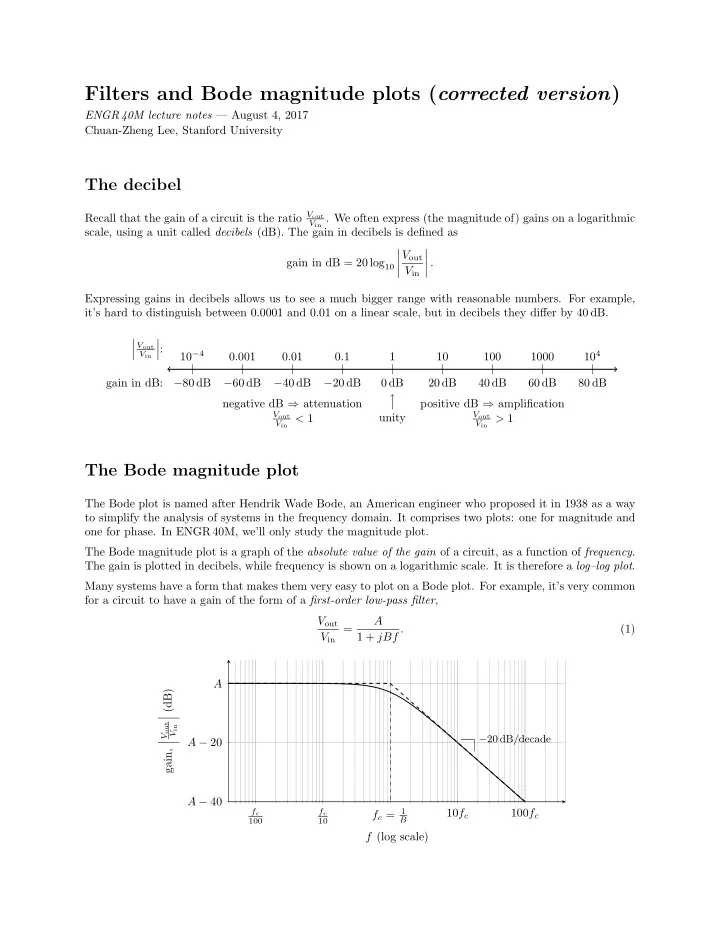
The Bode magnitude plot is a graph of the absolute value of the gain of a circuit, as a function of frequency. The gain is plotted in decibels, while frequency is shown on a logarithmic scale. It is therefore a log–log plot. Many systems have a form that makes them very easy to plot on a Bode plot. For example, it’s very common for a circuit to have a gain of the form of a first-order low-pass filter, Vout Vin = A 1 + jBf . (1)

fc 100 fc 10

fc = 1

B

10fc 100fc A − 40 A − 20 A

−20 dB/decade

f (log scale) gain,

• Vout

Vin

• (dB)

SLIDE 2

Another form commonly encountered is the first-order high-pass filter, Vout Vin = Af 1 + jBf . (2)

fc 100 fc 10

fc = 1

B

10fc 100fc

A B − 40 A B − 20 A B

20 dB/decade

f (log scale) gain,

• Vout

Vin

• (dB)

Asymptotes

Hendrik Wade Bode’s insight was that a log–log plot allows for an straight-line asymptotic approximation that is easy to draw and understand. You can find the asymptotes by taking, respectively, f → 0 and f → ∞, and then arguing that 1 ≫ Bf (in one case) or 1 ≪ Bf (in the other). When we say that 1 ≫ Bf, we mean that 1 is much greater than Bf, which implies that 1 + jBf ≈ 1; and the vice versa for 1 ≪ Bf. The power of the Bode plot, however, is that you don’t need to derive these asymptotes. A handful of salient features suffices to make the plot.

Important features

In a Bode plot of a first-order circuit, like the two forms above, there are three salient features that charac- terize the circuit. Generally, to draw a Bode plot, it suffices to find these three features. ❼ Horizontal asymptote. We find the horizontal asymptote as follows: – In a low-pass filter, we take f → 0 to get Vout

Vin ≈ A. This represents the DC gain.

– In a high-pass filter, we take f → ∞ to get Vout

Vin ≈ A B . This represents the high-frequency gain.

❼ Corner frequency (fc). Arguably the most defining characteristic, the corner frequency fc is where the two asymptotes intersect. It can be shown that this is equal to the frequency f at which the two additive terms in the denominator are equal (in magnitude). If you write your gain in the form (1) or (2), this frequency will be f = 1

B .

The corner frequency indicates where a filter stops “allowing” frequencies to pass through, i.e., where the gain starts to fall away from the maximum gain (horizontal asymptote). ❼ Slope of sloped asymptote. A “decade” is a multiplying of frequency by 10.1 Note that each decade is the same distance on the log-scaled frequency axis. – In a first-order low-pass filter, this is always −20 dB/decade. That is, each time you multiply frequency by 10, you divide gain by 10. – In a first-order high-pass filter, this is always 20 dB/decade. That is, each time you multiply frequency by 10, you multiply gain by 10. Note that, because of how log–log plots work, this slope doesn’t depend on A or B.

1A doubling of frequency is called an “octave”, named after the musical interval between two notes so related.

Then 20 dB/decade ≈ 6 dB/octave.

2

SLIDE 3

Filters

The low-pass filter described above in (1) is so named because it allows low frequencies to “pass through” with a gain of A, while attenuating high frequencies. Similarly, the high-pass filter in (2) allows high frequencies to pass through with a gain of A

B , while attenuating low frequencies.

There are two other types of filters: band-pass, which allows frequencies within a (finite) band and attenuates all frequencies outside that band, and band-stop, which attenuates frequencies within a (finite) band and allows all others. f (log scale) gain (dB) Low-pass filter f (log scale) gain (dB) High-pass filter f (log scale) gain (dB) Band-pass filter f (log scale) gain (dB) Band-stop filter Exercise 1. What do you think the ideal versions of each of the above types of filters would be? (Note: Ideal filters aren’t practically realizable.)

EveryCircuit

If you include an AC source in a circuit on EveryCircuit, you can get EveryCircuit to produce a Bode plot for the circuit by clicking the “Run AC” button. You’ll need to probe the output, just as you do for the time-based simulation. 3

SLIDE 4

Examples

Example 1. We return to the circuit in Example 1 from last lecture. vin(t) 10 kΩ 100 nF

+

− vout(t) Recall that the gain of this circuit was Vout Vin = 1 1 + j2πfRC = 1 1 + jf · 2π × 10−3 . (a) What are the corner frequency fc and DC gain of this circuit? (b) Draw a Bode plot for the gain Vout

Vin of this circuit.

(c) What type of filter is this? Example 2. We return to the circuit in Example 2 from last lecture. vin(t) 100 Ω 400 ➭H

+

− vout(t) Recall that the gain of this circuit was Vout Vin = j2πfL R + j2πfL = jf · 8π × 10−4 100 + jf · 8π × 10−4 . (a) What are the corner frequency fc and high-frequency gain of this circuit? Hint: It might be helpful to rearrange the expression above to make it conform with (2). (b) Draw a Bode plot for the gain Vout

Vin of this circuit.

(c) What type of filter is this? 4

SLIDE 5

Derivation of asymptotes

This is an supplement to the handout on filters and Bode magnitude plots.

Low-pass filter

Vout Vin = A 1 + jBf . Low-frequency asymptote. As f → 0, we have 1 ≫ Bf, so 1 + jBf ≈ 1. Then we have 20 log

• Vout

Vin

• = 20 log
• A

1 + jBf

• ≈ 20 log
• A

1

• = 20 log |A|,

that is, at low frequencies, the gain converges2 to the DC gain, whose magnitude is |A|. High-frequency asymptote. As f → ∞, 1 ≪ Bf, so 1 + jBf ≈ jBf. Then we have 20 log

• Vout

Vin

• = 20 log
• A

1 + jBf

• ≈ 20 log
• A

jBf

• = 20 log
• A

Bf

• = 20 log
• A

B

• − 20 log f,

that is, the high-frequency asymptote has a slope of −20 dB/decade (the coefficient of log f). Corner frequency. The asymptotes intersect where (assuming B is real and positive), 20 log |A| = 20 log

• A

Bfc

• = 20 log |A| − 20 log Bfc,

and solving this for fc yields fc = 1

B .

High-pass filter

Vout Vin = Af 1 + jBf . Low-frequency asymptote. As f → 0, we have 1 ≫ Bf, so 1 + jBf ≈ 1. Then we have 20 log

• Vout

Vin

• = 20 log
• Af

1 + jBf

• ≈ 20 log
• Af

1

• = 20 log |A| + 20 log f,

that is, the low-frequency asymptote has a slope of 20 dB/decade (the coefficient of log f). High-frequency asymptote. As f → ∞, 1 ≪ Bf, so 1 + jBf ≈ jBf. Then we have 20 log

• Vout

Vin

• = 20 log
• Af

1 + jBf

• ≈ 20 log
• Af

jBf

• = 20 log
• A

jB

• = 20 log
• A

B

• ,

that is, at high frequencies, the gain converges to the high-frequency gain, whose magnitude is 20 log

• A

B

• .

Corner frequency. The asymptotes intersect where (assuming B is real and positive), 20 log |Afc| = 20 log

• A

B

• ,

and solving this for fc yields fc = 1

B .

2Strictly speaking, our proof just shows that at lower frequencies, the gain is approximately the DC gain, not that it converges

to the DC gain. Nonetheless, the gain does in fact converge to the DC gain, and this isn’t too hard to prove (though we don’t require you to do so). A similar comment applies for every other place where the gain is approximately a constant.

5

SLIDE 6

Band-pass filter

Vout Vin = Af (1 + jBf)(1 + jCf). Analyzing this transfer function uses very similar ideas, there are just more terms to deal with. Here’s a

• guide. Filling in the gaps (in the same spirit as the low-pass and high-pass filters above) is left as an exercise.

Low-frequency asymptote. For the low-frequency asymptote, take f → 0 as usual, so that 1 ≫ Bf and 1 ≫ Cf. High-frequency asymptote. For the high-frequency asymptote, take f → ∞ as usual, so that 1 ≪ Bf and 1 ≪ Cf. Horizontal line in the middle. For this function, though, there is a “middle line”, which isn’t really an asymptote.3 This is nonetheless still part of the straight-line approximation. To find this middle approxima- tion, assume that f is in such a range such 1 dominates in one of the denominator terms, and the f term dominates in the other. For example, if B < C, assume that Bf ≪ 1 ≪ Cf. (This might not be a very good approximation, but it’s still insightful.) Your analysis should then yield a line that is horizontal on the Bode magnitude plot; that is, the passband of the filter. Corner frequencies. It then follows that there are two corner frequencies: one for the intersection between the low-frequency asymptote and the horizontal line, and one for the intersection between the horizontal line and the high-frequency asymptote.

3In order to qualify as an asymptote, the function has to get arbitrarily close to it.

6