
SLIDE 1
Example 1: First-Order Filters Consider the following filter: y[n] − ay[n − 1] = (1 − a)x[n]
- 1. Solve for the filter’s transfer function
- 2. Find the cutoff frequency as a function of a
Portland State University ECE 223 DT Filters
- Ver. 1.03
3
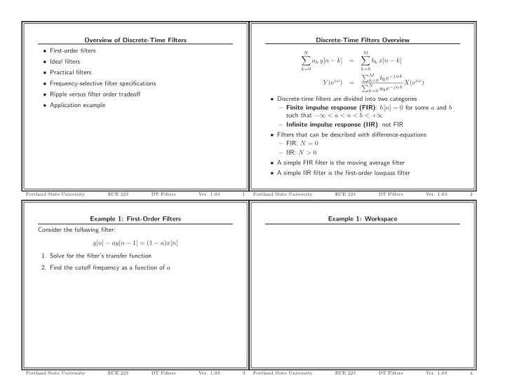
Overview of Discrete-Time Filters
- First-order filters
- Ideal filters
- Practical filters
- Frequency-selective filter specifications
- Ripple versus filter order tradeoff
- Application example
Portland State University ECE 223 DT Filters
- Ver. 1.03
1
Example 1: Workspace
Portland State University ECE 223 DT Filters
- Ver. 1.03
4
Discrete-Time Filters Overview
N
- k=0
ak y[n − k] =
M
- k=0
bk x[n − k] Y (ejω) = M
k=0 bke−jwk
N
k=0 ake−jwk X(ejω)
- Discrete-time filters are divided into two categories
– Finite impulse response (FIR): h[n] = 0 for some a and b such that −∞ < a < n < b < +∞ – Infinite impulse response (IIR): not FIR
- Filters that can be described with difference-equations
– FIR: N = 0 – IIR: N > 0
- A simple FIR filter is the moving average filter
- A simple IIR filter is the first-order lowpass filter
Portland State University ECE 223 DT Filters
- Ver. 1.03