Optimum IIR Filters Introduction and Scope Definitions Discussed - - PowerPoint PPT Presentation

optimum iir filters introduction and scope definitions
SMART_READER_LITE
LIVE PREVIEW

Optimum IIR Filters Introduction and Scope Definitions Discussed - - PowerPoint PPT Presentation

Optimum IIR Filters Introduction and Scope Definitions Discussed FIR filters for both stationary and nonstationary cases Design and properties For simplicity and due to time constraints, will limit discussion of IIR filters to


slide-1
SLIDE 1

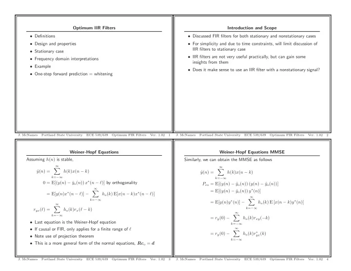
Weiner-Hopf Equations Assuming h(n) is stable, ˆ y(n) =

  • k=−∞

h(k)x(n − k) 0 = E[(y(n) − ˆ yo(n)) x∗(n − ℓ)] by orthogonality = E[y(n)x∗(n − ℓ)] −

  • k=−∞

ho(k) E[x(n − k)x∗(n − ℓ)] ryx(ℓ) =

  • k=−∞

ho(k)rx(ℓ − k)

  • Last equation is the Weiner-Hopf equation
  • If causal or FIR, only applies for a finite range of ℓ
  • Note use of projection theorem
  • This is a more general form of the normal equations, Rco = d
  • J. McNames

Portland State University ECE 539/639 Optimum FIR Filters

  • Ver. 1.02

3

Optimum IIR Filters

  • Definitions
  • Design and properties
  • Stationary case
  • Frequency domain interpretations
  • Example
  • One-step forward prediction = whitening
  • J. McNames

Portland State University ECE 539/639 Optimum FIR Filters

  • Ver. 1.02

1

Weiner-Hopf Equations MMSE Similarly, we can obtain the MMSE as follows ˆ y(n) =

  • k=−∞

h(k)x(n − k) Peo = E[(y(n) − ˆ yo(n)) (y(n) − ˆ yo(n))] = E[(y(n) − ˆ yo(n)) y∗(n)] = E[y(n)y∗(n)] −

  • k=−∞

ho(k) E [x(n − k)y∗(n)] = ry(0) −

  • k=−∞

ho(k)rxy(−k) = ry(0) −

  • k=−∞

ho(k)r∗

yx(k)

  • J. McNames

Portland State University ECE 539/639 Optimum FIR Filters

  • Ver. 1.02

4

Introduction and Scope

  • Discussed FIR filters for both stationary and nonstationary cases
  • For simplicity and due to time constraints, will limit discussion of

IIR filters to stationary case

  • IIR filters are not very useful practically, but can gain some

insights from them

  • Does it make sense to use an IIR filter with a nonstationary signal?
  • J. McNames

Portland State University ECE 539/639 Optimum FIR Filters

  • Ver. 1.02

2

slide-2
SLIDE 2

Impulse Response MSE Continued Pe = E [y∗(n)y(n)]

− E [y∗(n)ˆ y(n)]

− E [ˆ y∗(n)y(n)]

+ E [ˆ y∗(n)ˆ y(n)]

① = E [y∗(n)y(n)] = ry(0) = 1 2π π

−π

Ry(ejω) dω

  • J. McNames

Portland State University ECE 539/639 Optimum FIR Filters

  • Ver. 1.02

7

Weiner-Hopf Equations If noncasual IIR, the Weiner-Hopf equations apply for all values of ℓ and can be expressed as a convolution

  • k=−∞

ho(k)rx(ℓ − k) = ryx(ℓ) ho(ℓ) ∗ rx(ℓ) = ryx(ℓ) Ho(ejω)Rx(ejω) = Ryx(ejω) Ho = Ryx(ejω) Rx(ejω)

  • Thus we immediately obtain an expression for the optimal

noncausal transfer function

  • It is more difficult to obtain the optimum impulse response,

though it is completely defined by the Weiner-Hopf equations

  • J. McNames

Portland State University ECE 539/639 Optimum FIR Filters

  • Ver. 1.02

5

Impulse Response MSE Continued ② = E [y∗(n)ˆ y(n)] = E

  • y∗(n)
  • ℓ=−∞

h(ℓ)x(n − ℓ)

  • =

  • ℓ=−∞

h(ℓ) E [y∗(n)x(n − ℓ)] =

  • ℓ=−∞

h(ℓ)r∗

yx(ℓ) ∞

  • ℓ=−∞

h(ℓ)r∗

yx(ℓ)

= 1 2π ∞

−∞

H(ejω)R∗

yx(ejω) dω

③ = ②∗ = 1 2π ∞

−∞

H∗(ejω)Ryx(ejω) dω

  • J. McNames

Portland State University ECE 539/639 Optimum FIR Filters

  • Ver. 1.02

8

Impulse Response MSE Alternatively, we can minimize the MSE. Given that ˆ y(n) = h(n) ∗ x(n) where h(n) is not necessarily the optimal impulse response, find an expression for the MSE. Do not use the assumption that h(n) is FIR or causal in your derivation. Pe = E

  • |y(n) − ˆ

y(n)|2 = E

  • (y(n) − ˆ

y(n))∗ (y(n) − ˆ y(n))

  • =

E [(y∗(n) − ˆ y∗(n)) (y(n) − ˆ y(n))] = E [y∗(n)y(n)]

− E [y∗(n)ˆ y(n)]

− E [ˆ y∗(n)y(n)]

+ E [ˆ y∗(n)ˆ y(n)]

  • J. McNames

Portland State University ECE 539/639 Optimum FIR Filters

  • Ver. 1.02

6

slide-3
SLIDE 3

Impulse Response MSE Continued Pe = ry(0) −

  • ℓ=−∞

h(ℓ)r∗

yx(−ℓ) − ∞

  • ℓ=−∞

h∗(ℓ)ryx(−ℓ) +

  • k=−∞

h∗(k)

  • ℓ=−∞

h(ℓ)rx(k − ℓ) = 1 2π ∞

−∞

Ry(ejω) − H(ejω)R∗

yx(ejω) − H∗(ejω)Ryx(ejω)

+H∗(ejω)H(ejω)Rx(ejω) dω

  • Recall we did not assume h(n) is FIR or causal, though it does

work in the case

  • This gives us two additional ways of calculating the MSE in terms
  • f 1) the impulse response and 2) the frequency domain
  • J. McNames

Portland State University ECE 539/639 Optimum FIR Filters

  • Ver. 1.02

11

Impulse Response MSE Continued Pe = E [y∗(n)y(n)]

− E [y∗(n)ˆ y(n)]

− E [ˆ y∗(n)y(n)]

+ E [ˆ y∗(n)ˆ y(n)]

④ = E [ˆ y∗(n)ˆ y(n)] = E

  • k=−∞

h∗(k)x∗(n − k)

  • ℓ=−∞

h(ℓ)x(n − ℓ)

  • =

E

  • k=−∞

h∗(k)

  • ℓ=−∞

h(ℓ)x∗(n − k)x(n − ℓ)

  • =

  • k=−∞

h∗(k)

  • ℓ=−∞

h(ℓ) E [x(n − ℓ)x∗(n − k)] =

  • k=−∞

h∗(k)

  • ℓ=−∞

h(ℓ)rx(k − ℓ)

  • J. McNames

Portland State University ECE 539/639 Optimum FIR Filters

  • Ver. 1.02

9

Re-examining the Stationary MSE Recall that in the FIR case we can express the MSE in terms of the cross-correlation matrix R and vector d Pe = E

  • |e(n)|2

= E

  • y(n) − cHx(n)

H y(n) − cHx(n)

  • =

E

  • y∗(n) − xH(n)c

y(n) − cHx(n)

  • =

E

  • y∗(n)y(n) − xH(n)cy(n) − y∗(n)cHx(n)

+

  • cHx(n)

xH(n)c

  • =

E

  • |y(n)|2

− E

  • xH(n)y(n)
  • c − cH E [x(n)y∗(n)]

+cH E

  • x(n)xH(n)
  • c

= Py − dHc − cHd + cHRc where c∗ = h

  • J. McNames

Portland State University ECE 539/639 Optimum FIR Filters

  • Ver. 1.02

12

Impulse Response MSE Continued ④ =

  • k=−∞

h∗(k)

  • ℓ=−∞

h(ℓ)rx(k − ℓ) =

  • k=−∞

h∗(k) (h(k) ∗ rx(k)) z(k)

  • h(k) ∗ rx(k)

④ =

  • k=−∞

h∗(k)z(k) = 1 2π ∞

−∞

H∗(ejω)Z(ejω) dω = 1 2π ∞

−∞

H∗(ejω)H(ejω)Rx(ejω) dω

  • J. McNames

Portland State University ECE 539/639 Optimum FIR Filters

  • Ver. 1.02

10

slide-4
SLIDE 4

Frequency-Domain Minimum MSE If an optimum filter is used, Ho(ejω) = Ryx(ejω) Rx(ejω) then the MMSE is given by Peo = 1 2π π

−π

Ry(ejω) − Ho(ejω)R∗

yx(ejω) dω

= 1 2π π

−π

  • 1 − G2

yx(ω)

  • Ry(ejω) dω

where G2

yx(ω) is the magnitude squared coherence,

G2

yx(ω)

|Rxy(ejω)|2 Rx(ejω)Ry(ejω)

  • J. McNames

Portland State University ECE 539/639 Optimum FIR Filters

  • Ver. 1.02

15

Frequency Domain MSE: Completing the Square Find the optimum IIR noncausal H(ejω) by minimizing the MSE. Pe = 1 2π ∞

−∞

Ry(ejω) − H(ejω)R∗

yx(ejω) − Ryx(ejω)H∗(ejω)

+H(ejω)Rx(ejω)H∗(ejω) dω = 1 2π ∞

−∞

Ry(ejω) + H(ejω)

  • Rx(ejω)H∗(ejω) − R∗

yx(ejω)

  • −Ryx(ejω)H∗(ejω) dω

= 1 2π ∞

−∞

Ry(ejω) + Ryx(ejω)R−1

x (ejω)R∗ yx(ejω)

+

  • H(ejω) − Ryx(ejω)R−1

x (ejω)

Rx(ejω)H∗(ejω) − R∗

yx(ejω)

= 1 2π ∞

−∞

Ry(ejω) + Ryx(ejω)R−1

x (ejω)R∗ yx(ejω)

+

  • Rx(ejω)H(ejω) − Ryx(ejω)
  • R−1

x (ejω)

  • Rx(ejω)H(ejω) − Ryx(ejω)

∗ dω

  • J. McNames

Portland State University ECE 539/639 Optimum FIR Filters

  • Ver. 1.02

13

The Role of Coherence Po = 1 2π π

−π

  • 1 − G2

yx(ω)

  • Ry(ejω) dω
  • Recall that coherence is a measure of correlation in the frequency

domain

  • If coherence is 1 at a frequency, the error at that frequency is zero
  • Similarly, if incoherent, the error power is equal to the output

signal power

  • Applies to both causal IIR and FIR filters
  • J. McNames

Portland State University ECE 539/639 Optimum FIR Filters

  • Ver. 1.02

16

Optimum IIR Stationary Filter Pe = 1 2π ∞

−∞

Ry(ejω) + Ryx(ejω)R−1

x (ejω)R∗ yx(ejω)

+

  • Rx(ejω)H(ejω) − Ryx(ejω)
  • R−1

x (ejω)

  • Rx(ejω)H(ejω) − Ryx(ejω)

∗ dω

  • This is very similar to the approach we used to find the optimum

FIR filter in terms of R and d

  • The MMSE is obtained by setting the last term to zero,

Ho(ejω) = Ryx(ejω) Rx(ejω) as before Peo = 1 2π ∞

−∞

Ry(ejω) + Ho(ejω)R∗

yx(ejω) dω

  • Requires that Rx(ejω) be positive everywhere (no zeros on the

unit circle)

  • Equivalently, rx(ℓ) must be positive definite (strictly)
  • J. McNames

Portland State University ECE 539/639 Optimum FIR Filters

  • Ver. 1.02

14

slide-5
SLIDE 5

Optimum Causal Filter for White Input Signal Continued hyw,co(ℓ) = ryw(ℓ)

σ2

w

ℓ ≥ 0 ℓ < 0 Hyw,co(z) = 1 σ2

w

[Ryw(z)]+ [Ryw(z)]+

  • ℓ=0

ryw(ℓ)z−ℓ Pyw,co = ry(0) −

  • k=−∞

hyw,o(k)r∗

yw(k)

= ry(0) − 1 σ2

w ∞

  • ℓ=0

|ryw(ℓ)|2 where [·]+ denotes the one-sided z transform

  • J. McNames

Portland State University ECE 539/639 Optimum FIR Filters

  • Ver. 1.02

19

Causal IIR Filters

  • k

ho(k)rx(ℓ − k) = ryx(ℓ)

  • The solution we obtained before assumed no constraints
  • Solution is IIR and noncausal in general
  • We also know the solution for FIR filters in the stationary and

nonstationary cases

  • Historically, it was desirable to find the optimal causal IIR filter,

hco(ℓ) = 0 for ℓ < 0

  • Weiner-Hopf equations are no longer a convolution
  • The solution gives us some insight that we will use later
  • Note that

– A causal filter can be used to whiten any stationary process – If the input is white, the solution of the Weiner-Hopf equations in the causal case is trivial (next slide)

  • J. McNames

Portland State University ECE 539/639 Optimum FIR Filters

  • Ver. 1.02

17

Whitening the Input Signal Recall the spectral factorization theorem from last term (Section 2.4.4): If Rx(z) is analytic in a ring on the z plane that includes the unit circle, then Rx(z) can be factored as Rx(z) = σ2

wHx(z)H∗ x(z−∗)

where Hx(z) is a minimum-phase (i.e., stable, causal) system and x(n) = w(n) +

  • k=1

hx(k)w(n − k) X(z) = Hx(z)W(z) w(n) = x(n) −

  • k=1

hx(k)w(n − k) W(z) = H−1

x (z)X(z)

Here w(n) is linearly equivalent (i.e., there is a linear one-to-one mapping) with x(n). Therefore if we estimated y(n) using a linear combination of w(n) for n ≤ 0, it is possible to express this as a linear combination of x(n) for n ≤ 0.

  • J. McNames

Portland State University ECE 539/639 Optimum FIR Filters

  • Ver. 1.02

20

Optimum Causal Filter for White Input Signal Suppose we wish to find the optimal (noncausal, IIR) estimator for an input signal that is white, rw(ℓ) = σ2

wδ(ℓ),

ryw(ℓ) =

  • k=0

hco(k)rw(ℓ − k) =

  • k=0

hco(k)σ2

wδ(ℓ − k)

=

  • hco(ℓ)σ2

w

ℓ ≥ 0 ℓ < 0 hyw,co(ℓ) = ryw(ℓ)

σ2

w

ℓ ≥ 0 ℓ < 0

  • J. McNames

Portland State University ECE 539/639 Optimum FIR Filters

  • Ver. 1.02

18

slide-6
SLIDE 6

Remaining Tasks

  • Do an example similar to Example 6.6.1 in the text
  • Show that noncausal MMSE is significant less than the causal

MMSE, but the FIR MMSE approaches the causal MMSE with a modest filter order

  • Plot causal smoothing filter performance as a function of D to

demonstrate that not many samples are needed from the future to

  • btain an MMSE similar to the noncausal MMSE
  • J. McNames

Portland State University ECE 539/639 Optimum FIR Filters

  • Ver. 1.02

23

Combining the Two Steps: Whitening and Causal IIR Estimation Given the whitened signal, w(n), we know the optimal estimator is Hyw,co(z) = 1 σ2

w

[Ryw(z)]+ x(n) = hx(n) ∗ w(n) ryx(ℓ) = ryw(ℓ) ∗ h∗

x(−ℓ)

Ryx(z) = Ryw(z)H∗

x(z−∗)

Ryw(z) = Ryx(z) H∗

x(z−∗)

Hyw,co(z) = 1 σ2

x

Ryx(z) H∗

x(z−∗)

  • +

ˆ Y (z) = Hyw,co(z)W(z) W(z) = H−1

x (z)X(z)

Hco(z) = 1 σ2

wHx(z)

Ryx(z) H∗

x(z−∗)

  • +
  • J. McNames

Portland State University ECE 539/639 Optimum FIR Filters

  • Ver. 1.02

21

Causal IIR Prediction What is the one-step forward IIR linear predictor? y(n) x(n + 1) ˆ x(n + 1) =

  • k=0

hco(k)x(n − k) ˆ x(n) =

  • k=0

hco(k)x(n − 1 − k) ˆ X(z) = z−1HcoX(z) ef(n) = x(n) − ˆ x(n) HPEF(z) Ef(z) X(z) = X(z) − z−1HcoX(z) X(z) = 1 − z−1Hco(z)

  • J. McNames

Portland State University ECE 539/639 Optimum FIR Filters

  • Ver. 1.02

24

Comparison Ho(z) = Ryx(z) Rx(z) = 1 σ2

wHx(z)

Ryx(z) H∗

x(z−∗)

  • Hco(z) =

1 σ2

wHx(z)

Ryx(z) H∗

x(z−∗)

  • +

Peo = ry(0) − 1 σ2

x ∞

  • k=−∞

|ryw(k)|2 Peco = ry(0) − 1 σ2

x ∞

  • k=0

|ryw(k)|2

  • The noncausal MMSE is called the irreducible MMSE because it

is the best performance that can be achieved by a linear filter

  • Both can be viewed as a whitening filter followed by an optimum

causal filter for a white input

  • J. McNames

Portland State University ECE 539/639 Optimum FIR Filters

  • Ver. 1.02

22

slide-7
SLIDE 7

Wold Decomposition Theorem Revisited e(n) = hPEF(n) ∗ x(n) HPEF(z) = 1 Hx(z) Peo = 1 2π π

−π

|HPEF(ejω)|2Rx(ejω) dω

  • A random process x(n) is predictable if Peo = 0
  • Only processes with line spectrum (i.e., harmonic processes =

PSD consists of a sum of impulses) are predictable

  • Sometimes called deterministic processes
  • Due to the idea that the prediction error filter can only be exactly

zero at a finite number of frequencies (zeros on the unit circle)

  • Wold decomposition theorem tells us every random process can be

decomposed into a regular component with a continuous PSD and a predictable process (line spectra)

  • J. McNames

Portland State University ECE 539/639 Optimum FIR Filters

  • Ver. 1.02

27

Causal IIR Prediction Continued Solve for Hco(z) when y(n) = x(n + 1) ryx(ℓ) = rx(ℓ + 1) Ryx(z) = zRx(z) Hco(z) =

  • n=0

hco(n)z−n = 1 σ2

wHx(z)

Ryx(z) H∗

x(z−∗)

  • +

= 1 σ2

wHx(z)

zRx(z) H∗

x(z−∗)

  • +

= 1 σ2

wHx(z)

zσ2

wHx(z)H∗ x(z−∗)

H∗

x(z−∗)

  • +

= [zHx(z)]+ Hx(z) = zHx(z) − zhx(0) Hx(z)

  • J. McNames

Portland State University ECE 539/639 Optimum FIR Filters

  • Ver. 1.02

25

Causal IIR Prediction Continued HPEF(z) = 1 − z−1Hco(z) = 1 − z−1 zHx(z) − zhx(0) Hx(z) = Hx(z) Hx(z) − Hx(z) − hx(0) Hx(z) = 1 Hx(z)

  • This is the same expression we had for our whitening filter!
  • The one-step IIR linear predictor is identical to the minimum

phase whitening filter of the process!

  • The prediction errors ef(n) = x(n) − ˆ

x(n) are therefore white

  • The prediction error filter is minimum phase
  • The MMSE is σ2

w as long as hx(0) 1

  • J. McNames

Portland State University ECE 539/639 Optimum FIR Filters

  • Ver. 1.02

26