
SLIDE 1
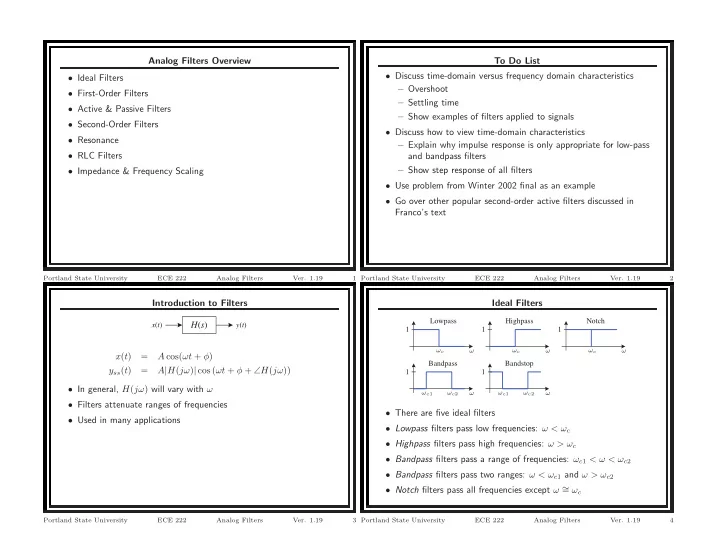
Introduction to Filters H(s)
x(t) y(t)
x(t) = A cos(ωt + φ) yss(t) = A|H(jω)| cos (ωt + φ + ∠H(jω))
- In general, H(jω) will vary with ω
- Filters attenuate ranges of frequencies
- Used in many applications
Portland State University ECE 222 Analog Filters
- Ver. 1.19
3
Analog Filters Overview
- Ideal Filters
- First-Order Filters
- Active & Passive Filters
- Second-Order Filters
- Resonance
- RLC Filters
- Impedance & Frequency Scaling
Portland State University ECE 222 Analog Filters
- Ver. 1.19
1
Ideal Filters
1 Lowpass 1 Highpass 1 Bandpass 1 Bandstop 1 Notch
ω ω ω ω ω ωc ωc ωc ωc1 ωc1 ωc2 ωc2
- There are five ideal filters
- Lowpass filters pass low frequencies: ω < ωc
- Highpass filters pass high frequencies: ω > ωc
- Bandpass filters pass a range of frequencies: ωc1 < ω < ωc2
- Bandpass filters pass two ranges: ω < ωc1 and ω > ωc2
- Notch filters pass all frequencies except ω ∼
= ωc
Portland State University ECE 222 Analog Filters
- Ver. 1.19
4
To Do List
- Discuss time-domain versus frequency domain characteristics
– Overshoot – Settling time – Show examples of filters applied to signals
- Discuss how to view time-domain characteristics
– Explain why impulse response is only appropriate for low-pass and bandpass filters – Show step response of all filters
- Use problem from Winter 2002 final as an example
- Go over other popular second-order active filters discussed in
Franco’s text
Portland State University ECE 222 Analog Filters
- Ver. 1.19