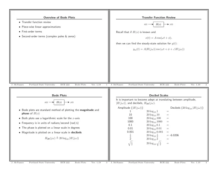
overview of bode plots transfer function review transfer
play

Overview of Bode Plots Transfer Function Review Transfer function - PowerPoint PPT Presentation

Overview of Bode Plots Transfer Function Review Transfer function review x ( t ) H ( s ) y ( t ) Piece-wise linear approximations First-order terms Recall that if H ( s ) is known and Second-order terms (complex poles & zeros) x


  1. Overview of Bode Plots Transfer Function Review • Transfer function review x ( t ) H ( s ) y ( t ) • Piece-wise linear approximations • First-order terms Recall that if H ( s ) is known and • Second-order terms (complex poles & zeros) x ( t ) = A cos( ωt + φ ) , then we can find the steady-state solution for y ( t ) : y ss ( t ) = A | H ( jω ) | cos ( ωt + φ + ∠ H ( jω )) J. McNames Portland State University ECE 222 Bode Plots Ver. 1.19 1 J. McNames Portland State University ECE 222 Bode Plots Ver. 1.19 2 Bode Plots Decibel Scales It is important to become adept at translating between amplitude, H ( s ) x ( t ) y ( t ) | H ( jω ) | , and decibels, H dB ( jω ) . Amplitude ( | H ( jω ) | ) Decibels ( 20 log 10 | H ( jω ) | ) • Bode plots are standard method of plotting the magnitude and 1 20 log 10 1 = phase of H ( s ) 10 20 log 10 10 = 100 20 log 10 100 = • Both plots use a logarithmic scale for the x -axis 1000 20 log 10 1000 = • Frequency is in units of radians/second (rad/s) 0.1 20 log 10 0 . 1 = • The phase is plotted on a linear scale in degrees 0.01 20 log 10 0 . 01 = 0.001 20 log 10 0 . 001 = • Magnitude is plotted on a linear scale in decibels 1 1 20 log 10 = -6.0206 2 2 H dB ( jω ) � 20 log 10 | H ( jω ) | 2 20 log 10 2 = � � 1 1 20 log 10 = 2 2 J. McNames Portland State University ECE 222 Bode Plots Ver. 1.19 3 J. McNames Portland State University ECE 222 Bode Plots Ver. 1.19 4

  2. Example 1: Bode Plots Example 1: Workspace 20 nF 10 k Ω 1 k Ω + v s ( t ) v o ( t ) R L - 1. Find the transfer function of the circuit shown above. 2. Generate the bode plot. J. McNames Portland State University ECE 222 Bode Plots Ver. 1.19 5 J. McNames Portland State University ECE 222 Bode Plots Ver. 1.19 6 Example 1: Bode Plot Example 1: MATLAB Code w = logspace(1,5,500); Active Lowpass RC Filter H = -50e3./(j*w + 5e3); 20 |H(j ω )| (dB) subplot(2,1,1); h = semilogx(w,20*log10(abs(H))); set(h,’LineWidth’,1.4); 10 ylabel(’|H(j\omega)| (dB)’); title(’Active Lowpass RC Filter’); 0 set(gca,’Box’,’Off’); grid on; 1 2 3 4 5 set(gca,’YLim’,[-5 25]); 10 10 10 10 10 subplot(2,1,2); 180 h = semilogx(w,angle(H)*180/pi); ∠ H(j ω ) (degrees) set(h,’LineWidth’,1.4); 160 ylabel(’\angle H(j\omega) (degrees)’); set(gca,’Box’,’Off’); 140 grid on; 120 set(gca,’YLim’,[85 185]); 100 xlabel(’Frequency (rad/s)’); 1 2 3 4 5 10 10 10 10 10 Frequency (rad/s) J. McNames Portland State University ECE 222 Bode Plots Ver. 1.19 7 J. McNames Portland State University ECE 222 Bode Plots Ver. 1.19 8

  3. Example 2: Bode Plots Example 2: Workspace 1 µ F 2 µ F 1 k Ω 1 k Ω + v s ( t ) R L - 1. Find the transfer function of the circuit shown above. 2. Generate the bode plot. J. McNames Portland State University ECE 222 Bode Plots Ver. 1.19 9 J. McNames Portland State University ECE 222 Bode Plots Ver. 1.19 10 Example 2: Bode Plot Example 2: MATLAB Code w = logspace(1,5,500); Active Lead/Lag RC Filter 8 H = -2*(j*w+500)./(j*w + 1000); 6 |H(j ω )| (dB) subplot(2,1,1); h = semilogx(w,20*log10(abs(H))); 4 set(h,’LineWidth’,1.4); 2 ylabel(’|H(j\omega)| (dB)’); title(’Active Lead/Lag RC Filter’); 0 set(gca,’Box’,’Off’); grid on; −2 1 2 3 4 5 set(gca,’YLim’,[-2 8]); 10 10 10 10 10 subplot(2,1,2); −160 h = semilogx(w,angle(H)*180/pi); ∠ H(j ω ) (degrees) set(h,’LineWidth’,1.4); −165 ylabel(’\angle H(j\omega) (degrees)’); set(gca,’Box’,’Off’); −170 grid on; set(gca,’YLim’,[-180 -160]); −175 −180 xlabel(’Frequency (rad/s)’); 1 2 3 4 5 10 10 10 10 10 Frequency (rad/s) J. McNames Portland State University ECE 222 Bode Plots Ver. 1.19 11 J. McNames Portland State University ECE 222 Bode Plots Ver. 1.19 12

  4. Bode Plot Approximations Alternate Transfer Function Expressions There are many equivalent expressions for transfer functions. • Until recently (late 1980’s) bode plots were drawn by hand N ( s ) • There were many rules-of-thumb, tables, and template plots to H ( s ) = help D ( s ) b m s m + b m − 1 s m − 1 + · · · + b 1 s + b 0 • Today engineers primarily use MATLAB, or the equivalent = a n s n + a n − 1 s n − 1 + · · · + a 1 s + a 0 • Why discuss the old method of plotting by hand? b m s ± ℓ ( s − z 1 )( s − z 2 ) . . . ( s − z m ) – It is still important to understand how the poles, zeros, and = a n ( s − p 1 )( s − p 2 ) . . . ( s − p n ) gain influence the Bode plot � � � � � � 1 − s 1 − s s – These ideas are used for transfer function synthesis, analog . . . 1 − z 1 z 2 z m k s ± ℓ = circuit design, and control systems � � � � � � 1 − s 1 − s s . . . 1 − p 1 p 2 p n • We will discuss simplified methods of generating Bode plots • Based on asymptotic approximations • This last expression is called standard form • The first step in making bode plots is to convert H ( s ) to standard form J. McNames Portland State University ECE 222 Bode Plots Ver. 1.19 13 J. McNames Portland State University ECE 222 Bode Plots Ver. 1.19 14 Magnitude Components Magnitude Components Comments Consider the expression for the transfer function magnitude: | H dB ( ω ) | = 20 log 10 | k | ± ℓ 20 log 10 ω | H dB ( jω ) | = 20 log 10 | H ( jω ) | � � � � � 1 − jω � 1 − jω +20 log 10 � + · · · + 20 log 10 � � � � z 1 z m � � s ± ℓ (1 − s s � z 1 ) . . . (1 − z m ) � � = 20 log 10 � � � � � k � � � 1 − jω � 1 − jω − 20 log 10 � − · · · − 20 log 10 (1 − s s p 1 ) . . . (1 − p n ) � � � � � � p 1 p n � � s = jω 20 log 10 | k | · | jω | ± ℓ | 1 − jω z 1 | . . . | 1 − jω • Thus, | H dB ( ω ) | can be written as a sum of simple functions z m | = | 1 − jω p 1 | . . . | 1 − jω p n | • This is similar like using basis functions { δ ( t ) , u ( t ) ,& r ( t ) } to write an expression for a piecewise linear signal = 20 log 10 | k | ± ℓ 20 log 10 ω • We will use this approach to generate our piecewise linear � � � � � 1 − jω � 1 − jω � � � � +20 log 10 � + · · · + 20 log 10 approximations of the bode plot � � � � z 1 z m � � � � � • Note that there are four types of components in this expression � 1 − jω � 1 − jω � � � � − 20 log 10 � − · · · − 20 log 10 – Constant – Linear term � � � � p 1 p n � – Zeros – Poles J. McNames Portland State University ECE 222 Bode Plots Ver. 1.19 15 J. McNames Portland State University ECE 222 Bode Plots Ver. 1.19 16

  5. Magnitude Components: Constant Magnitude Components: Linear Term (dB) (dB) | H ( jω ) | | H ( jω ) | 40 40 20 20 0 0 (rad/sec) (rad/sec) ω ω -20 -20 -40 -40 The constant term, 20 log 10 | k | , is a straight line on the Bode plot. The linear term, ± ℓ 20 log 10 | ω | , is a line on the magnitude plot with a slope equal to ± ℓ 20 dB per decade. The x -axis intercept occurs at ω = 1 rad/s. Plot the bode magnitude plots for H ( s ) = s , 1 s , s 2 , 1 s 2 . J. McNames Portland State University ECE 222 Bode Plots Ver. 1.19 17 J. McNames Portland State University ECE 222 Bode Plots Ver. 1.19 18 Magnitude Components: Real Zeros Magnitude Components: Real Zeros Continued Consider two limiting conditions for a term containing a zero, | H ( jω ) | (dB) � 1 − jω � � 20 log 10 � z 40 First condition: ω ≪ | z | 20 � 1 − jω � = 0 � � z → 0 20 log 10 lim z ω 0 (rad/sec) ω � 1 − jω � ≈ 0 . ω � � Thus, if | z | ≪ 1 , then 20 log 10 -20 z Second condition: ω ≫ | z | -40 � = 20 log 10 | − jω � � 1 − jω � z →∞ 20 log 10 lim z | = 20 log 10 | ω | − 20 log 10 | z | z ω Our piecewise approximation joins these two linear asymptotic approximations at ω = | z | . ω Thus, if | z | ≫ 1 , then this term is linear (on a log scale) with a slope � 1 − jω � � of 20 dB per decade and an x -axis intercept at ω = | z | . Plot the piecewise approximation of the term 20 log 10 � . z J. McNames Portland State University ECE 222 Bode Plots Ver. 1.19 19 J. McNames Portland State University ECE 222 Bode Plots Ver. 1.19 20

Download Presentation
Download Policy: The content available on the website is offered to you 'AS IS' for your personal information and use only. It cannot be commercialized, licensed, or distributed on other websites without prior consent from the author. To download a presentation, simply click this link. If you encounter any difficulties during the download process, it's possible that the publisher has removed the file from their server.

Recommend


More recommend