Transfer Functions Transfer Functions Assume zero initial - PowerPoint PPT Presentation

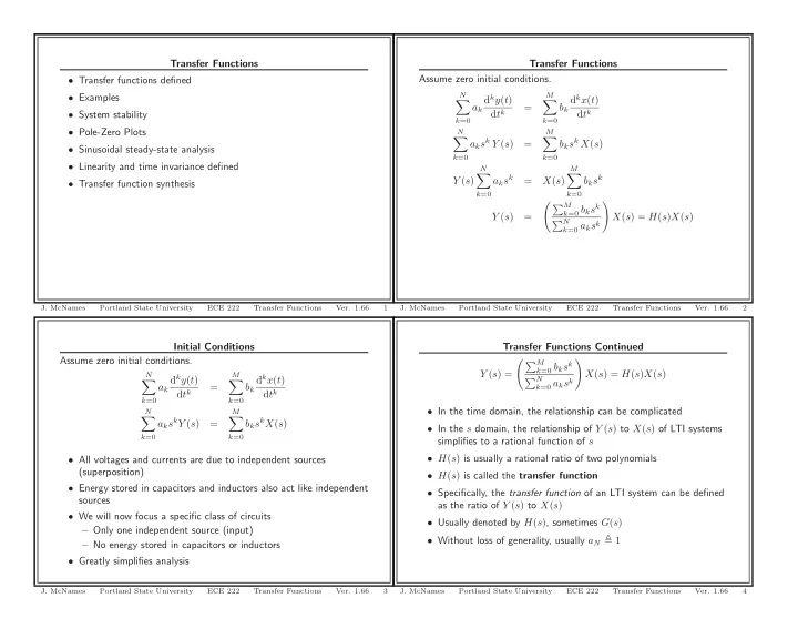
Transfer Functions Transfer Functions Assume zero initial conditions. • Transfer functions defined N M • Examples d k y ( t ) d k x ( t ) � � a k = b k d t k d t k • System stability k =0 k =0 • Pole-Zero Plots N M a k s k Y ( s ) b k s k X ( s ) � � = • Sinusoidal steady-state analysis k =0 k =0 • Linearity and time invariance defined N M � a k s k � b k s k Y ( s ) = X ( s ) • Transfer function synthesis k =0 k =0 � � M � k =0 b k s k Y ( s ) = X ( s ) = H ( s ) X ( s ) � N k =0 a k s k J. McNames Portland State University ECE 222 Transfer Functions Ver. 1.66 1 J. McNames Portland State University ECE 222 Transfer Functions Ver. 1.66 2 Initial Conditions Transfer Functions Continued Assume zero initial conditions. � � M � k =0 b k s k Y ( s ) = X ( s ) = H ( s ) X ( s ) N M d k y ( t ) d k x ( t ) � N k =0 a k s k � � a k = b k d t k d t k k =0 k =0 • In the time domain, the relationship can be complicated N M � � a k s k Y ( s ) b k s k X ( s ) = • In the s domain, the relationship of Y ( s ) to X ( s ) of LTI systems k =0 k =0 simplifies to a rational function of s • H ( s ) is usually a rational ratio of two polynomials • All voltages and currents are due to independent sources (superposition) • H ( s ) is called the transfer function • Energy stored in capacitors and inductors also act like independent • Specifically, the transfer function of an LTI system can be defined sources as the ratio of Y ( s ) to X ( s ) • We will now focus a specific class of circuits • Usually denoted by H ( s ) , sometimes G ( s ) – Only one independent source (input) • Without loss of generality, usually a N � 1 – No energy stored in capacitors or inductors • Greatly simplifies analysis J. McNames Portland State University ECE 222 Transfer Functions Ver. 1.66 3 J. McNames Portland State University ECE 222 Transfer Functions Ver. 1.66 4

Example 1: Transfer Function vs. Impulse Response Transfer Functions and the Impulse Response Fill in the missing parts to determine how the transfer function of an h ( t ) x ( t ) y ( t ) H ( s ) x ( t ) y ( t ) LTI system G ( s ) is related to the impulse response h ( t ) x ( t ) = δ ( t ) X ( s ) = • Because of their relationship, both H ( s ) and h ( t ) completely y ( t ) = Y ( s ) = characterize the LTI system L − 1 { G ( s ) } = L { h ( t ) } = • If the LTI system is a circuit, once you know either H ( s ) or h ( t ) , you have sufficient information to calculate the output • You now have three different approaches to solve for the output of an LTI circuit – y ( t ) = x ( t ) ∗ h ( t ) – Solve for H ( s ) , X ( s ) , and then y ( t ) = L − 1 { H ( s ) X ( s ) } – Use Laplace transform circuit analysis to solve for the outputs of interest • All three have limitations, advantages, and disadvantages J. McNames Portland State University ECE 222 Transfer Functions Ver. 1.66 5 J. McNames Portland State University ECE 222 Transfer Functions Ver. 1.66 6 Continous-Time Convolution Tradeoffs Transfer Function Analysis Tradeoffs h ( t ) x ( t ) y ( t ) H ( s ) x ( t ) y ( t ) h ( t ) x ( t ) y ( t ) H ( s ) x ( t ) y ( t ) Transfer Function: y ( t ) = L − 1 { H ( s ) X ( s ) } Continuous-time Convolution: y ( t ) = x ( t ) ∗ h ( t ) • Advantages • Advantages – Can find solution for all t , not just t > 0 – Reduces differential equation to an algebra problem – Can be approximated using discrete-time convolution – Usually the easiest approach • Disadvantages – Easy to find the output for different input signals – Cannot account for non-zero initial conditions, requires • Disadvantages complete x ( t ) and y ( t ) – Can only solve for y ( t ) for t > 0 – Can be difficult to write and solve integrals – Requires zero initial conditions – Can only be used for single-input single-output (SISO) systems – Can only be used for SISO systems J. McNames Portland State University ECE 222 Transfer Functions Ver. 1.66 7 J. McNames Portland State University ECE 222 Transfer Functions Ver. 1.66 8

Laplace Transform Circuit Analysis Tradeoffs Example 6: Transfer Functions R h ( t ) x ( t ) y ( t ) H ( s ) x ( t ) y ( t ) + Laplace Transform Circuit Analysis v s ( t ) C v o ( t ) • Advantages - – Elegant method of handling non-zero initial conditions – Can handle multiple sources (multiple inputs) & can solve for Find the transfer function for the circuit above. The input is the multiple outputs (any voltage or current) — MIMO systems voltage source v s ( t ) and the output is labeled v o ( t ) . • Disadvantages – Can only solve for y ( t ) for t > 0 – Cannot account for full history, x ( t ) for t < 0 . Requires this effect to be captured in the initial conditions – Can be tedious – Specific to application (circuits), we did not discuss generalization to other types of systems J. McNames Portland State University ECE 222 Transfer Functions Ver. 1.66 9 J. McNames Portland State University ECE 222 Transfer Functions Ver. 1.66 10 Example 7: Transfer Functions Example 8: Transfer Functions R C C R + + v s ( t ) v s ( t ) v o ( t ) v o ( t ) - - Find the transfer function for the circuit above. Do you recognize this Find the transfer function for the circuit above. Do you recognize this function? function? J. McNames Portland State University ECE 222 Transfer Functions Ver. 1.66 11 J. McNames Portland State University ECE 222 Transfer Functions Ver. 1.66 12

Example 9: Transfer Functions Example 9: Workspace C B C A R B R A + v s ( t ) v o ( t ) R L - Find the transfer function for the circuit above. J. McNames Portland State University ECE 222 Transfer Functions Ver. 1.66 13 J. McNames Portland State University ECE 222 Transfer Functions Ver. 1.66 14 Example 10: Transfer Functions Example 10: Workspace v R ( t ) v L ( t ) + - + - R L + v s ( t ) C v C ( t ) - Find the transfer function from the input voltage to an output voltage across each element of the three passive elements in a series RLC circuit. J. McNames Portland State University ECE 222 Transfer Functions Ver. 1.66 15 J. McNames Portland State University ECE 222 Transfer Functions Ver. 1.66 16

Poles and Stability Pole-Zero Plots Assume all of the poles in a transfer function H ( s ) are unique. Then H ( s ) = N ( s ) H ( s ) can be written as follows using partial fraction expansion: D ( s ) N N ( s ) k ℓ � • Zeros : roots of N ( s ) H ( s ) = D ( s ) = s − p ℓ • Poles : roots of D ( s ) ℓ =1 N • Poles must be in the left half plane for the system to be stable L − 1 { H ( s ) } � k ℓ e + p ℓ t u ( t ) = h ( t ) = • As the poles get closer to the boundary, the system becomes less ℓ =1 stable • Note the expansion is in terms of the poles, rather than − p ℓ � ∞ • Pole-Zero Plot : plot of the zeros and poles on the complex s • If −∞ | h ( t ) | d t < ∞ , the LTI system is bounded-input plane bounded-output (BIBO) stable • You will use these throughout the junior sequence (ECE 32x) • That is | h ( t ) | < α < ∞ for all t • h ( t ) is bounded if Re { p ℓ } < 0 for all ℓ • The system is BIBO stable if and only if all the poles are in the left half of the complex plane J. McNames Portland State University ECE 222 Transfer Functions Ver. 1.66 17 J. McNames Portland State University ECE 222 Transfer Functions Ver. 1.66 18 Example 11: Pole-Zero Plots Example 11: Pole-Zero Plot Use MATLAB to generate a Pole-Zero plot for a system with the Pole−Zero Plot 1.5 following transfer function s 2 − 1 1 H ( s ) = s 3 + 4 s 2 + 6 s + 4 Using the MATLAB, we can quickly find the roots 0.5 Imaginary Axis ( s + 1)( s − 1) H ( s ) = 0 ( s + 2)( s + 1 − j )( s + 1 + j ) Is the system stable? The pole-zero plot, impulse response, and step −0.5 response are shown on the following slides. −1 −1.5 −3 −2.5 −2 −1.5 −1 −0.5 0 0.5 1 1.5 2 Real Axis J. McNames Portland State University ECE 222 Transfer Functions Ver. 1.66 19 J. McNames Portland State University ECE 222 Transfer Functions Ver. 1.66 20

Example 11: MATLAB Code for Pole-Zero Plot Example 11: Impulse Response sys = tf([1 0 -1],[1 4 6 4]); Impulse Response figure; [p,z] = pzmap(sys); 1 h = plot(real(p),imag(p),’bx’,real(z),imag(z),’ro’); set(h,’LineWidth’,1.2); 0.8 set(h,’MarkerSize’,5); hold on; plot([0 0],[-2 2],’k:’,[-3 2],[0 0],’k:’); 0.6 hold off; xlabel(’Real Axis’); 0.4 h(t) ylabel(’Imaginary Axis’); title(’Pole-Zero Plot’); 0.2 axis([-3 2 -1.5 1.5]); 0 −0.2 −0.4 0 1 2 3 4 5 6 7 Time (seconds) J. McNames Portland State University ECE 222 Transfer Functions Ver. 1.66 21 J. McNames Portland State University ECE 222 Transfer Functions Ver. 1.66 22 Example 11: MATLAB Code for Impulse Response Example 11: Step Response sys = tf([1 0 -1],[1 4 6 4]); Step Response figure; t = 0:0.01:7; 0.1 [h,t] = impulse(sys,t); h = plot(t,h); set(h,’LineWidth’,1.5); 0 hold on; plot([0 0],[-2 2],’k:’,[0 max(t)],[0 0],’k:’); hold off; −0.1 axis([0 max(t) -0.5 1.2]); y(t) xlabel(’Time (seconds)’); ylabel(’h(t)’); −0.2 title(’Impulse Response’); −0.3 −0.4 −0.5 0 1 2 3 4 5 6 7 Time (seconds) J. McNames Portland State University ECE 222 Transfer Functions Ver. 1.66 23 J. McNames Portland State University ECE 222 Transfer Functions Ver. 1.66 24