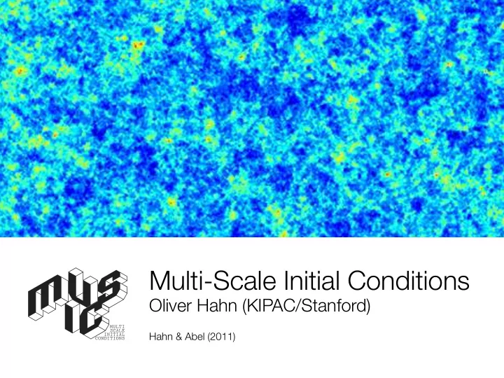
Oliver Hahn (KIPAC/Stanford)
Hahn & Abel (2011)
Multi-Scale Initial Conditions
MULTI SCALE INITIAL CONDITIONS

Multi-Scale Initial Conditions Oliver Hahn (KIPAC/Stanford) MULTI - - PowerPoint PPT Presentation
Multi-Scale Initial Conditions Oliver Hahn (KIPAC/Stanford) MULTI SCALE Hahn & Abel (2011) INITIAL CONDITIONS Some pre-to-post-CMB physics: Inflation leads to near scale-invariant primordial density spectrum P prim ( k )
Hahn & Abel (2011)
MULTI SCALE INITIAL CONDITIONS
Oliver Hahn SC comparison workshop 08/2012 Multi-scale ICs
Inflation leads to near scale-invariant primordial density spectrum Gets processed by growth on sub- and super-horizon scales (GR): Multi-species fluid of CDM+baryon+photon+neutrino →linear Boltzmann solver (e.g. Ma & Bertschinger 1995)
10
−4
10
−2
10 10
2
10
−4
10
−2
10 10
2
10
4
10
6
comoving k [h/Mpc] T(k) z=200000 z=20000 z=2000 z=200 z=20
super-horizon sub-horizon
radiation-dom. matter-dom.
Oliver Hahn SC comparison workshop 08/2012 Multi-scale ICs
Identify the peak (or region) from which an object forms e.g. cluster halo at z=0 corresponding peak patch in white noise field We want to increase the resolution locally in this patch... 1:1 mapping
Oliver Hahn SC comparison workshop 08/2012 Multi-scale ICs
Gaussian density perturbation field:
galaxy, cluster, first star...
environment, sample variance
(cf. Bertschinger 2001, GRAFIC-2)
Oliver Hahn SC comparison workshop 08/2012 Multi-scale ICs
because that’s where the peak patch lives... Remember the generation of a density field with given power spectrum:
real space TF Gaussian white noise What does it mean?
(cf. also Salmon 1996)
Oliver Hahn SC comparison workshop 08/2012 Multi-scale ICs
The T(r) kernel for baryons over cosmic time:
20 40 60 80 100 120 140 160 −1 −0.5 0.5 1 1.5 2 2.5 3 x 10
−6
comoving radius [Mpc/h] δ (r) z=2000 z=1400 z=1000
Propagating wave for z>1000 Convolution superimposes waves and growing modes on noise.
sound speed ~ c/3
20 40 60 80 100 120 140 160 −1 −0.5 0.5 1 1.5 2 2.5 3 x 10
−6
comoving radius [Mpc/h] δ (r) z=1000 z=700 z=500
Stalled wave for z<1000
sound speed drops after recomb perturbations grow
Linear regime: no interaction between waves.
Oliver Hahn SC comparison workshop 08/2012 Multi-scale ICs
Advantages:
Ω1
a) top grid 2N b) subgrid
Ω
p
N
Ω
Ω2 Ω2,p Multi-scale convolutions relatively easy to deal with: sample “propagator” at different resolutions important: need to be locally-mass conserving
Oliver Hahn SC comparison workshop 08/2012 Multi-scale ICs
Lagrangian perturbation theory relates density perturbations to displacements and velocities
x(t) = q + L(q, t), ˙ x(t) = d dtL(q, t) (
need to solve Poisson’s equation adaptive multi-grid (Fedorenko 1961, Brandt 1973,1977) can achieve this on nested grids. But uses finite differences! straightforward to generalize to 2LPT L(q) ∝ rqΦ(q, t) at 1st order, displacement field is proportional to gravitational force (Zel’dovich 1970)
Oliver Hahn SC comparison workshop 08/2012 Multi-scale ICs
Order n Laplacian L Gradient G exact: ∂2
x
∂x 2: ⇥ 1 2 1 ⇤
1 2
⇥ 1 1 ⇤ 4:
1 12
⇥ 1 16 30 16 1 ⇤
1 12
⇥ 1 8 8 1 ⇤ 6:
1 180
⇥ 2 27 270 490 270 27 2 ⇤
1 60
⇥ 1 9 45 45 9 1 ⇤ exact: k2 i k 2: 2 [ cos(k) + 1] i sin(k) 4: 1
6 [cos(2k) 16 cos(k) + 15]
i
6 [ sin(2k) + 8 sin(k)]
6: 1
90 [2 cos(3k) + 27 cos(2k) 270 cos(k) + 245]
i
30 [sin(3k) 9 sin(2k) + 45 sin(k)]
j(k) =
⇧ i kj k2 − G(n)
j
L(n) ⌃
Keep long-range, inter-grid interaction from multi-grid
Oliver Hahn SC comparison workshop 08/2012 Multi-scale ICs
1 level, error in std. dev of the field 2 level, error in std. dev of the field
Oliver Hahn SC comparison workshop 08/2012 Multi-scale ICs
degraded, hybrid multi-scale, hybrid 1 level 2 level T(r), hybrid
To test, refine region just around the cluster peak patch
See José Oñorbe’s talk for details about errors related to the choice of Lagrangian region and resolution...
Oliver Hahn SC comparison workshop 08/2012 Multi-scale ICs
Mvir, Rvir, Vmax, spin parameter, 3D velocity dispersion, shape parameters <1% errors in gross halo properties
Oliver Hahn SC comparison workshop 08/2012 Multi-scale ICs
Gadget-2
1283 base resolution, 100 Mpc/h box
Gadget-2
3 levels = 5123 effective
Gadget-2
3 levels + adiabatic gas RAMSES ENZO 2 levels + adiabatic gas
Oliver Hahn SC comparison workshop 08/2012 Multi-scale ICs
103 104 105 106 107 108 109 Number of particles per halo 100 101 102 103 104 105 106 Number of halos (per 0.1 dex of mass)
Rhapsody 4k Rhapsody 8k Phoenix Aquarius
Consuelo Carmen Bolshoi MultiDark Millennium Millennium-XXL
Wu et al. 2012a/b, to be submitted
Oliver Hahn SC comparison workshop 08/2012 Multi-scale ICs
A Web Interface
and stored as ASCII files.
Clicking on the correlation matrix brings you to the scatter plots. Mark red points (halos) in a specified range. Browse history and sharing key. Each point represent one
show the image of the
in red. Choose two halo properties to show a scatter plot.
[Implemented by Yao-Yuan Mao]
Oliver Hahn SC comparison workshop 08/2012 Multi-scale ICs
Oliver Hahn SC comparison workshop 08/2012 Multi-scale ICs
Full public access probably in September
Gadget, ENZO, RAMSES, Gasoline (ART in progress)
fitting formulae
errors with grid codes
resolution, enlarge region...