Figure 11.1 An 8-puzzle problem instance: (a) initial configuration; - - PDF document

figure 11 1 an 8 puzzle problem instance a initial
SMART_READER_LITE
LIVE PREVIEW

Figure 11.1 An 8-puzzle problem instance: (a) initial configuration; - - PDF document

5 2 1 2 3 1 8 3 4 5 6 4 7 6 7 8 (a) (b) 5 2 1 5 2 1 5 2 1 5 2 1 5 2 up up left down 1 8 3 8 3 4 8 3 4 8 3 4 3 4 7 6 4 7 6 7 6 7 6 7 8 6 left down 1 2 3 1 2 3 1 2 1 2 up up


slide-1
SLIDE 1

(a) Blank tile (b) Last tile moved (c) 1 4 1 4 2 7 7 8 5 2 3 3 8 5 1 6 3 6 6 8 6 3 2 5 8 7 6 3 4 5 8 7 4 1 2 4 1 7 6 5 2 5 7 4 8 1 7 6 3 2 5 4 4 8 1 5 7 6 3 2 2 2 4 8 1 5 7 6 3 2 3 4 8 1 5 6 7 3 2 3 4 8 1 5 7 6 8 1 up up left left down down left up up

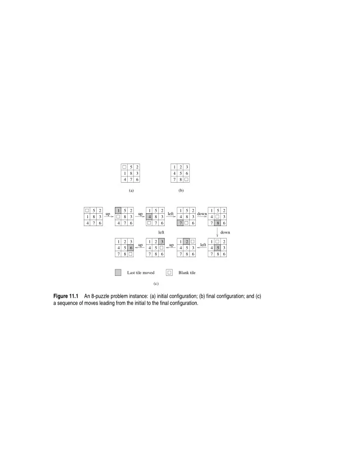
Figure 11.1 An 8-puzzle problem instance: (a) initial configuration; (b) final configuration; and (c) a sequence of moves leading from the initial to the final configuration.

slide-2
SLIDE 2

Non-terminal node Terminal node (goal) Terminal node (non-goal)

x1 = 0 x1 = 1 x2 = 0 x2 = 1 x3 = 0 x3 = 0 x3 = 1 x3 = 1 x4 = 0 x4 = 0 x4 = 1 x4 = 1 f (x) = 0 f (x) = 2

Figure 11.2 The graph corresponding to the 0/1 integer-linear-programming problem.

slide-3
SLIDE 3

(a)

4 3 2 1 3 1 2 4 5 6 7 8 10 9 8 3 2 6 4 4 5 6 5 7 7 7 7

(b)

8 9 10 10 9 10 10 8 9 8 1 10 10 9 10 10 2 9 8 7 9 8 7 6 7 9 8 6 5 4 3 1 5

Figure 11.3 Two examples of unfolding a graph into a tree.

slide-4
SLIDE 4

8 7 1 6 5 4 2 4 3 1 6 5 8 2 7 4 8 7 3 6 5 2 3 4 8 7 1 6 5 2 1 7 1 6 5 3 8 2 3 4 8 7 1 5 6 2 3 4 8 7 1 6 5 4 4 8 7 1 6 5 3 2 3 2

A D E F G H C B

down down right up up right right

The last tile moved Blank tile Step 3 Step 2 Step 1

Figure 11.4 States resulting from the first three steps of depth-first search applied to an instance

  • f the 8-puzzle.
slide-5
SLIDE 5

(c) (a) (b)

15 16 17 20 18 19 21 22 23 24 1 2 7 8 9 10 11 12 13 14 Bottom of the stack 11 Top of the stack Current State 3 5 4 5 4 9 8 11 14 19 14 17 16 19 24 23 6 5 4 3 1 24 23 21 18 15 17 16 13 10 7 9 8

Figure 11.5 Representing a DFS tree: (a) the DFS tree; successor nodes shown with dashed lines have already been explored; (b) the stack storing untried alternatives only; and (c) the stack storing untried alternatives along with their parent. The shaded blocks represent the parent state and the block to the right represents successor states that have not been explored.

slide-6
SLIDE 6

(a) (c) (b)

2 3 4 7 1 6 5 8 2 3 4 8 7 1 6 5 2 3 4 8 7 1 6 5 7 6 7 Step 1 2 3 4 8 7 1 6 5 2 3 4 8 7 1 6 5 2 3 4 7 1 6 5 8 2 4 8 7 1 6 5 3 2 3 4 8 7 1 5 6 2 3 4 7 1 5 6 3 4 8 7 1 5 6 2 3 8 7 1 5 6 8 2 4 6 7 7 Step 2 8 6 7 7 7 Step 1 2 3 4 8 7 1 6 5 1 2 3 4 5 6 7 8 The last tile moved Blank Tile 2 3 4 8 7 1 6 5 2 8 7 1 6 5 2 3 4 7 1 6 5 8 2 3 4 8 7 1 5 2 4 8 7 1 6 6 5 3 6 7 Step 2 7 8 6 Step 1 2 3 4 7 6 5 8 1 2 3 4 8 7 1 6 5 2 3 4 8 7 1 6 5 2 3 4 7 1 6 5 8 3 2 3 4 7 1 5 8 6 7 2 4 8 7 1 6 5 3 2 3 4 8 7 1 5 6 2 3 4 7 1 5 6 3 4 8 7 1 5 6 2 3 8 7 1 5 6 8 2 4 6 7 Step 2 Step 4 8 6 8 7 7 7 8 Step 1 Step 3 4

Figure 11.6 Applying best-first search to the 8-puzzle: (a) initial configuration; (b) final configura- tion; and (c) states resulting from the first four steps of best-first search. Each state is labeled with its h-value (that is, the Manhattan distance from the state to the final state).

slide-7
SLIDE 7

C E F B A (a) (b) D

Figure 11.7 The unstructured nature of tree search and the imbalance resulting from static parti- tioning.

slide-8
SLIDE 8

Service any pending messages Do a fixed amount of work Select a processor and request work from it Service any pending messages Finished available work Got work Issued a request Got a reject Processor idle Processor active

Figure 11.8 A generic scheme for dynamic load balancing.

slide-9
SLIDE 9

(a) (b)

14 4 3 16 14 13 10 8 7 1 4 8 16 5 23 24 19 17 11 9 1 7 9 10 11 13 15 17 18 19 21 22 23 24 3 5

Cutoff depth Current State

Figure 11.9 Splitting the DFS tree in Figure 11.5. The two subtrees along with their stack repre- sentations are shown in (a) and (b).

slide-10
SLIDE 10

Step 1 Step 3 Step 5 Step 2 Step 6 Step 4

w0 = 0.5 w0 = 0.5 w0 = 0.5 w0 = 0.25 w0 = 0.25 w0 = 1.0 w1 = 0.5 w1 = 0.5 w1 = 0.5 w1 = 0.25 w1 = 0.25 w2 = 0.25 w2 = 0.25 w3 = 0.25 w3 = 0.25

Figure 11.10 Tree-based termination detection. Steps 1–6 illustrate the weights at various pro- cessors after each work transfer.

slide-11
SLIDE 11

100 200 300 400 500 600 700 200 400 600 800 1000 1200 ARR GRR RP

p Speedup

Figure 11.11 Speedups of parallel DFS using ARR, GRR and RP load-balancing schemes.

slide-12
SLIDE 12

GRR Expected (GRR) RP Expected (RP) 100000 300000 500000 700000 900000 200 400 600 800 1000 1200

p Number of work requests

Figure 11.12 Number of work requests generated for RP and GRR and their expected values (O(p log2 p) and O(p log p) respectively).

slide-13
SLIDE 13

1.5e+07 2e+07 2.5e+07 5e+06 1e+07 E = 0.74 E = 0.85 E = 0.90 E = 0.64 20000 40000 60000 80000 100000 120000

W p log p

2

Figure 11.13 Experimental isoefficiency curves for RP for different efficiencies.

slide-14
SLIDE 14

Number of busy Processors Number of busy Processors Number of busy Processors Time (a) (b) (c) Time Time

Figure 11.14 Three different triggering mechanisms: (a) a high triggering frequency leads to high load-balancing cost, (b) the optimal frequency yields good performance, and (c) a low frequency leads to high idle times.

slide-15
SLIDE 15

Idle Busy 1 2 3 4 5 6 4 3 2 1 7 6 5 Global pointer Global pointer

Figure 11.15 Mapping idle and busy processors with the use of a global pointer.

slide-16
SLIDE 16

Expand the node to generate successors Expand the node to generate successors Expand the node to generate successors at designated processor Global list maintained best node nodes Put expanded Get current Pick the best node from the list Place generated nodes in the list Pick the best node from the list Place generated nodes in the list Unlock the list Pick the best node from the list Place generated nodes in the list Unlock the list Unlock the list Lock the list Lock the list Lock the list

P0 P1 Pp−1 Figure 11.16 A general schematic for parallel best-first search using a centralized strategy. The locking operation is used here to serialize queue access by various processors.

slide-17
SLIDE 17

Exchange best nodes Exchange best nodes Exchange best nodes Local list Local list Local list

P0 P1 Pp−1 Figure 11.17 A message-passing implementation of parallel best-first search using the ring com- munication strategy.

slide-18
SLIDE 18

Exchange best nodes Exchange best nodes Local list Local list Local list

blackboard

Exchange best nodes

P0 P1 Pp−1 Figure 11.18 An implementation of parallel best-first search using the blackboard communication strategy.

slide-19
SLIDE 19

Start node S Start node S (a)

1 2 3 5 6 7

Total number of nodes generated by sequential formulation = 13 Total number of nodes generated by (b) Goal node G Goal node G two-processor formulation of DFS = 9

9 12 10 4 8 11 13 R1 R3 L2 L3 L1 R2 R4 R5 L4

Figure 11.19 The difference in number of nodes searched by sequential and parallel formulations

  • f DFS. For this example, parallel DFS reaches a goal node after searching fewer nodes than se-

quential DFS.

slide-20
SLIDE 20

L1 L2 L3 L4 L5 R7 R6 R5 R4 R3 R1 R2 1 2 3 4 5 6 7 Total number of nodes generated by (a) (b) Total number of nodes generated by Start node S Start node S Goal node G Goal node G sequential DFS = 7 two-processor formulation of DFS = 12

Figure 11.20 A parallel DFS formulation that searches more nodes than its sequential counterpart.

slide-21
SLIDE 21

x+2 1 2 x+3 x+4 x+1 1 1 1 1 1 1 Initially, x+2 1 3 2 x+1 x x x+3 After Increment, x x+2

000 001 010 100 110 101 111 011

target target = x+5

000 001 010 011 100 101 110 111 000 000 100 000 010 100 110

= x

Figure 11.21 Message combining and a sample implementation on an eight-processor hypercube.

slide-22
SLIDE 22

(manager) Processors Search tree Subtasks Subtask generator Work request

Figure 11.22 The single-level work-distribution scheme for tree search.