Family of intersection problems Family of intersection problems CG - - PDF document

SLIDE 1

1

1

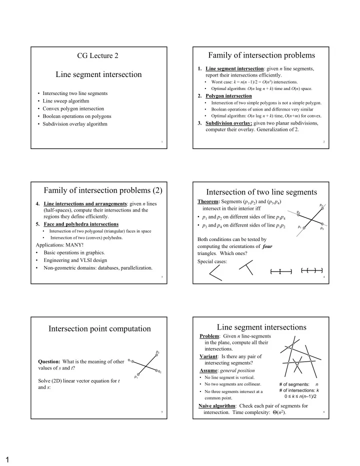
CG Lecture 2 CG Lecture 2

Line segment intersection

• Intersecting two line segments
• Line sweep algorithm
• Convex polygon intersection
• Boolean operations on polygons
• Subdivision overlay algorithm

2

Family of intersection problems Family of intersection problems

• 1. Line segment intersection: given n line segments,

report their intersections efficiently.

• Worst case: k = n(n –1)/2 = O(n2) intersections.
• Optimal algorithm: O(n log n + k) time and O(n) space.
• 2. Polygon intersection
• Intersection of two simple polygons is not a simple polygon.
• Boolean operations of union and difference very similar
• Optimal algorithm: O(n log n + k) time, O(n+m) for convex.
• 3. Subdivision overlay: given two planar subdivisions,

computer their overlay. Generalization of 2.

3

Family of intersection problems (2) Family of intersection problems (2)

• 4. Line intersections and arrangements: given n lines

(half-spaces), compute their intersections and the regions they define efficiently.

• 5. Face and polyhedra intersections
• Intersection of two polygonal (triangular) faces in space
• Intersection of two (convex) polyhedra.

Applications: MANY!

• Basic operations in graphics.
• Engineering and VLSI design
• Non-geometric domains: databases, parallelization.

4

Intersection of two line segments Intersection of two line segments

Theorem: Segments (p1,p2) and (p3,p4) intersect in their interior iff

• p1 and p2 on different sides of line p3p4
• p3 and p4 on different sides of line p1p2

Both conditions can be tested by computing the orientations of four

• triangles. Which ones?

Special cases:

p4 p2 p3 p1

5

Intersection point computation Intersection point computation

1 2 1 1 2 1

( ) ( ) 1 ( ) ( ) 1 p t p p p t t q s q q q s s = + − ≤ ≤ = + − ≤ ≤

q1 p2 q2 p1

Question: What is the meaning of other values of s and t? Solve (2D) linear vector equation for t and s: ( ) ( ) [0,1] [0,1] p t q s t s = ∈ ∈

check that and

6

Line segment intersections Line segment intersections

Problem: Given n line-segments in the plane, compute all their intersections. Variant: Is there any pair of intersecting segments? Assume: general position

• No line segment is vertical.
• No two segments are collinear.
• No three segments intersect at a

common point.

Naive algorithm: Check each pair of segments for

• intersection. Time complexity: Θ(n2).

# of segments: # of segments: n n # of intersections: # of intersections: k k 0 ≤ ≤ k k ≤ ≤ n n( (n n– –1)/2 1)/2

SLIDE 2

2

7

Line segment intersections Line segment intersections

Goal: Output-sensitive algorithm

• O(n log n + k log n) time
• O(n) space
• not optimal, but good start

Idea:

• Segments that are close

together are candidates for intersection.

• Keep track of “closedness”

changes.

If x and y projections If x and y projections don don’ ’t intersect, t intersect, no intersection. no intersection.

8

Sweep line: idea Sweep line: idea

Segment adjacencies with respect to a horizontal (vertical) line change locally:

• si and sj must be adjacent for

the intersection to occur.

• (si,sj) before intersection.
• (sj,si) after intersection.

Keep track of segment adjacencies as vertical line moves from left to right. Stop only at event points!

s1 s2 s3 s5 s4 s6 (s1,s2,s3) (s1,s3,s2) (s1,s3)

9

Adjacency theorem Adjacency theorem

Theorem: Just before an intersection

• ccurs (infinitesimally-close to it),

the two respective segments are adjacent to each other in the sweep-line status. Proof: In practice: Look ahead: whenever two line segments become adjacent along the sweep line, check for their intersection below the sweep line.

10

Sweep line algorithm Sweep line algorithm

• An event is any endpoint or

intersection point.

• Sweep a horizontal line from top

to bottom. Maintain two data structures:

• Event priority queue Q: sorted by

y coordinate.

• Sweep line status L: stores

segments currently intersected by the sweep line, sorted by y coordinate.

# of events # of events ≤ ≤ n n + + k k # of segments in # of segments in L L ≤ ≤ n n s1 s2 s3 s5 s4 s6 () (s2,s3) (s2)

11

Balanced binary tree Balanced binary tree

• Balanced binary tree sorted by x coordinate
• Insertion, deletion, and neighbor operations in O(log n)

s1 s4 s1 s2 s3 s1 s4 s2 s3 s2 s5 s4 s3 s5

12

Sweep line algorithm Sweep line algorithm

Initialization:

• Put all segment endpoints in the event queue Q,

sorted according to y coordinates. Time: O(n log n).

• Sweep line status is initially empty.

The algorithm proceeds by inserting, deleting, and handling discrete events from the queue Q until it is

• empty. It also maintains the list L.

SLIDE 3

3

13

Event handling Event handling – – start of segment start of segment

Event of type A: Beginning of segment (upper endpoint)

• Locate segment position in the status.
• Insert segment into sweep line status.
• Test for intersection below the sweep

line with the segments immediately to the left and right of it. Insert intersection point(s) (if found, and if not already in the queue) into the event queue.

Time complexity: n events, O(log n) time for each → O(n log n) total.

si sj sk sl

14

Event handling Event handling – – end of segment end of segment

Event of type B: End of segment (lower endpoint)

• Locate segment position in the status.
• Delete segment from sweep line status.
• Test for intersection below the sweep line

between the segments immediately to the left and right. Insert intersection point (if found, and if not already in the queue) into the event queue.

Time complexity: n events, O(log n) time for each → O(n log n) in total.

si sj sk sl

15

Event handling Event handling – – intersection intersection

Event of type C: Intersection point

• Report the point.
• Swap the two respective line segments in

the sweep line status.

• For the new left and right segments – test

each for intersection against the segment immediately adjacent the status line (if exists). Insert intersection point (if found, and if not already in the queue) into the event queue.

Time complexity: k such events, O(log n)

each → O(k log n) in total. k is the k is the

• utput size
• utput size

si sj sl sm

16

Example Example

s4 s2 s1 s0 s3 e1 Sweep Line Status Event Queue a1 b 1 a0 b0 a2 b2 a4 a3 b3 b4

17

Complexity analysis Complexity analysis

• Basic data structures:
• Event queue: heap
• Sweep line status: balanced binary tree
• Each heap/tree operation requires O(log n) time.

(Why is O(log k) = O(log n) ?)

• Total time complexity: O((n+k) log n).
• If k≈n2 this is slightly worse than the naive algorithm.
• When k=o(n2/log n) then the sweep algorithm is faster.
• Total space complexity: O(n+k).

Question: How can this be improved to O(n)?

• Note: There exists a better algorithm whose running

time is Θ(n log n + k) with O(n+k) space complexity.

18

Handling Handling degeneracies degeneracies

• Horizontal segments with

same y coordinate treat them in arbitrary order (i.e., from left to right y coordinate)

• Overlapping segments

report them as special

• Multiple segment

intersections at the same point

si p q si p sj sk si p sj

SLIDE 4

4

19

Handling Handling degeneracies degeneracies

20

Line segment intersection algorithm Line segment intersection algorithm

21

Intersection of convex polygons Intersection of convex polygons

Input: Two convex polygons |A| = n and |B| = m. Output: one convex polygon |A ∩ B| ≤ n + m in optimal O(n+m) time and space. Observations:

• alternation of A and B boundary

pieces.

• alternation at intersection points
• rder of vertices is kept.
• at each intersection, choose

leftmost segment. 4 1 2 5 3 6 8 7 9 10 11 A = A = { {1,2,3,4,5 1,2,3,4,5} } B B = { = {6,7,8,9 6,7,8,9} } I I = { = {10,11 10,11} } A A ∩ ∩ B B = { = {6,7 6,7, ,10 10, ,8,9 8,9, ,11 11} }

22

Code for convex polygon intersection Code for convex polygon intersection

23

Advance rules Advance rules

Do not advance on the boundary of either A or B whose Do not advance on the boundary of either A or B whose current edge may contain a yet current edge may contain a yet-

• to

to-

• be

be-

• found intersection

found intersection ai bj advance ai bj advance ai bj advance ai bj advance

24

Example of convex intersection trace Example of convex intersection trace

a a b b

SLIDE 5

5

25

Binary operations on polygons Binary operations on polygons

Operations: intersection, union, difference. Observations:

• Operations on simple connected

polygons can lead to holes and disconnected pieces

• Operations are similar, once the

intersection points are found. Only the boundary reconstruction rules changes.

• Maximum number of

pieces/holes is O(nm)

6 7 8 1 2 3 4 5

A A B B

A = A = { {1,2,3,4,5 1,2,3,4,5} } B B = { = {6,7,8 6,7,8} } I I = { = {9,10,11,12,13,14 9,10,11,12,13,14} } 9 9 10 10 11 11 12 12 13 13 14 14

26

Maximum number of pieces/holes Maximum number of pieces/holes

Each piece has Each piece has O O( (n n) slabs. ) slabs. The intersection has O( The intersection has O(n n2

2) pieces.

) pieces.

27

Intersection of polygons Intersection of polygons

6 7 8 1 2 3 4 5

A A B B

A = A = { {1,2,3,4,5 1,2,3,4,5} } B B = { = {6,7,8 6,7,8} } I I = { = {9,10,11,12,13,14 9,10,11,12,13,14} } A A ∩ ∩ B B = { = {9,10,11,12} 9,10,11,12} U U { {13,3,14 13,3,14} } 9 9 10 10 11 11 12 12 13 13 14 14 3

A A ∩ ∩ B B

9 9 10 10 11 11 13 13 14 14 Boundary rule Boundary rule: : Follow segment with Follow segment with both both interiors to the left interiors to the left 12 12

28

Union of polygons Union of polygons

6 7 8 1 2 3 4 5

A A B B

A = A = { {1,2,3,4,5 1,2,3,4,5} } B B = { = {6,7,8 6,7,8} } I I = { = {9,10,11,12,13,14 9,10,11,12,13,14} } A A U UB B = {( = {(6,10,1,11,8,7,14,4,5), 6,10,1,11,8,7,14,4,5),( (9,2,13) 9,2,13)} } 9 9 10 10 11 11 12 12 13 13 14 14 7 A A U U B B 9 9 10 10 11 11 13 13 14 14 Boundary rule Boundary rule: : Follow segment with Follow segment with either interior to the left either interior to the left 6 6 1 1 8 8 4 5 2 2

29

Difference of polygons Difference of polygons

6 7 8 1 2 3 4 5

A A B B

A = A = { {1,2,3,4,5 1,2,3,4,5} } B B = { = {6,7,8 6,7,8} } I I = { = {9,10,11,12,13,14 9,10,11,12,13,14} } A A – – B B = { = {9,12,2,13,14,4,5 9,12,2,13,14,4,5} } 9 9 10 10 11 11 12 12 13 13 14 14 A A – – B B 9 9 12 12 13 13 14 14 Boundary rule: Boundary rule: Follow segment with Follow segment with A A’ ’s interior to the left s interior to the left 4 5 2 2

30

Subdivision overlay intersection Subdivision overlay intersection

Algorithm for a more general class of shapes subdivision overlays, a subdivision of faces in the plane represented by a planar graph. Idea: use the sweep line technique to detect intersections and build the new overlay by adding vertices and updating pointers.

• Start with an overlay consisting of

two disconnected components, S1 and S2.

• Add points and links as events occur.

S S2

2

S S1

1

O(S O(S1

1,S

,S2

2)

)

SLIDE 6

6

31

Subdivision overlay representation Subdivision overlay representation

A face is the maximal connected A face is the maximal connected subset of the plane that does not subset of the plane that does not contain in its interior a point on an edge contain in its interior a point on an edge

• r vertex. The incident edges and
• r vertex. The incident edges and

vertices form its boundary. vertices form its boundary. Representation as a doubly Representation as a doubly-

• connected

connected edge list. Directed edges are half edge list. Directed edges are half-

• edges

edges

• Vertex

Vertex: coordinates, incident edge : coordinates, incident edge

• Face

Face: inner and outer components : inner and outer components

• Half

Half-

• edge

edge: origin, twin edge, next : origin, twin edge, next and previous edges, incident face. and previous edges, incident face.

32

Example of subdivision Example of subdivision

33

Event handling Event handling – – sketch sketch

• Use a sweep line, stopping at vertices. Keep a doubly

Use a sweep line, stopping at vertices. Keep a doubly connected list connected list D D, initially containing edges of , initially containing edges of S S1

1 and

and S S2

2

• If the event involves only edges from either

If the event involves only edges from either S S1

1 or

• r S

S2

2,

, there is no need to update there is no need to update D. D.

• Otherwise, locally update the data structures.

Otherwise, locally update the data structures. (pointer manipulations (pointer manipulations – – tedious details omitted). tedious details omitted).

• All operations take

All operations take O O( (m m) ), , where where m m is the cardinality is the cardinality

• f the vertex.
• f the vertex.
• At the end of the sweep line, the vertex and edges have

At the end of the sweep line, the vertex and edges have been properly handled in the data structure. been properly handled in the data structure.

• The face information (old and new faces) must now be

The face information (old and new faces) must now be updated to create updated to create O O( (S S1

1,S

,S2

2).

).

34

Event handling Event handling – – example example

v v1

1

v v2

2

u u4

4

u u3

3

v v1

1

u u4

4

u u3

3

v v2

2

w w5

5

e e12

12

e e21

21

e e43

43

e e34

34

e e15

15

e e52

52

35

Boundary and face tracing Boundary and face tracing

• Boundary cycles are extracted directly from D by

following pointers faces are directly created and extracted.

• Missing information: is the boundary an outer or

an inner face? Which face does it belong to?

• Inner or outer face: find the angle of the leftmost
• vertex. If it is greater than π, then it is an outer

face, otherwise it is an outer face.

36

Face handling Face handling – – connected components connected components

holes holes

• uter boundaries
• uter boundaries

SLIDE 7

7

37

Subdivision intersection algorithm (1) Subdivision intersection algorithm (1)

• 1. Initialize D with S1 and S2
• 2. Compute all intersections between edges from S1 and

edges of S2 with line-sweep. In addition to the actions on T and Q, do

• 1. Update D when the event involves edges from both S1 and S2.
• 2. Store first half-edge to the left of the event point at

corresponding vertex in D (used later for face computation).

• 3. Find boundary cycles.
• 4. Compute connected components of graph G whose

nodes are boundary cycles and whose arcs connect each hole cycle to the cycle left of its leftmost vertex.

38

Subdivision intersection algorithm (2) Subdivision intersection algorithm (2)

• 5. For each connected component in G do:

Let C be the unique outer boundary cycle in the component, and let f be the face bounded by the cycle.

• a. Create a face record for f
• b. Set OuterComponent(f) to a half-edge of C
• c. Construct the list InnerComponents(f) with pointers to
• ne half-edge in each hole cycle in the component.
• d. Make the IncidentFace() pointers of all half-edges in

the cycles point to the face record of f.

Theorem Theorem: The overlay of two planar subdivisions : The overlay of two planar subdivisions S S1

1 and

and S S2

2

• f complexity
• f complexity n

n can be computed in can be computed in O O( (n nlog logn n + + k klog logn n) where ) where k k is the complexity of is the complexity of the resulting overlay. the resulting overlay.

39

Line segment intersection algorithms Line segment intersection algorithms

• Naïve O(n2)
• Bentley-Ottman, 1988: O((n+k) log n)
• Edelsbrunner-Chazelle, 1990: O(nlogn + k)

requires O(nlogn) space, complex.

• Clarkson-Shor, Mumuley, 1992:

O(nlogn + k) with randomized O(n) space

• Balaban, 1995: O(nlogn + k)

with O(n) space, optimal deterministic. Solved a long open problem!