discrete random variables probability mass function given
play

Discrete random variables Probability mass function Given a discrete - PDF document

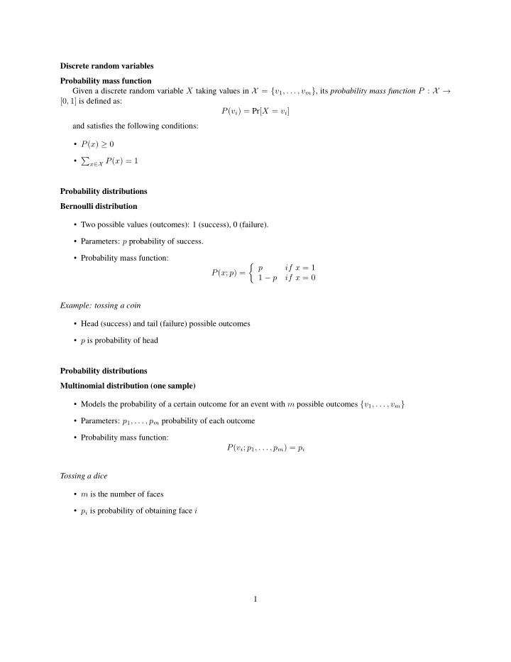
Discrete random variables Probability mass function Given a discrete random variable X taking values in X = { v 1 , . . . , v m } , its probability mass function P : X [0 , 1] is defined as: P ( v i ) = Pr [ X = v i ] and satisfies the


  1. Discrete random variables Probability mass function Given a discrete random variable X taking values in X = { v 1 , . . . , v m } , its probability mass function P : X → [0 , 1] is defined as: P ( v i ) = Pr [ X = v i ] and satisfies the following conditions: • P ( x ) ≥ 0 • � x ∈X P ( x ) = 1 Probability distributions Bernoulli distribution • Two possible values (outcomes): 1 (success), 0 (failure). • Parameters: p probability of success. • Probability mass function: � if x = 1 p P ( x ; p ) = 1 − p if x = 0 Example: tossing a coin • Head (success) and tail (failure) possible outcomes • p is probability of head Probability distributions Multinomial distribution (one sample) • Models the probability of a certain outcome for an event with m possible outcomes { v 1 , . . . , v m } • Parameters: p 1 , . . . , p m probability of each outcome • Probability mass function: P ( v i ; p 1 , . . . , p m ) = p i Tossing a dice • m is the number of faces • p i is probability of obtaining face i 1

  2. Continuouos random variables Probability density function Instead of the probability of a specific value of X , we model the probability that x falls in an interval ( a, b ) : � b Pr [ x ∈ ( a, b )] = p ( x ) dx a Properties: • p ( x ) ≥ 0 � ∞ −∞ p ( x ) dx = 1 • Note The probability of a specific value x 0 is given by: 1 p ( x 0 ) = lim ǫ Pr [ x ∈ [ x 0 , x 0 + ǫ )] ǫ → 0 Probability distributions Gaussian (or normal) distribution • Bell-shaped curve. • Parameters: µ mean, σ 2 variance. • Probability density function: 2 πσ exp − ( x − µ ) 2 1 p ( x ; µ, σ ) = √ 2 σ 2 2

  3. • Standard normal distribution: N (0 , 1) • Standardization of a normal distribution N ( µ, σ 2 ) z = x − µ σ Conditional probabilities conditional probability probability of x once y is observed P ( x | y ) = P ( x, y ) P ( y ) statistical independence variables X and Y are statistical independent iff P ( x, y ) = P ( x ) P ( y ) implying: P ( x | y ) = P ( x ) P ( y | x ) = P ( y ) Basic rules law of total probability The marginal distribution of a variable is obtained from a joint distribution summing over all possible values of the other variable ( sum rule ) � � P ( x ) = P ( x, y ) P ( y ) = P ( x, y ) y ∈Y x ∈X product rule conditional probability definition implies that P ( x, y ) = P ( x | y ) P ( y ) = P ( y | x ) P ( x ) Bayes’ rule P ( y | x ) = P ( x | y ) P ( y ) P ( x ) Playing with probabilities Use rules! • Basic rules allow to model a certain probability given knowledge of some related ones • All our manipulations will be applications of the three basic rules • Basic rules apply to any number of varables: � � P ( y ) = P ( x, y, z ) (sum rule) x z � � P ( y | x, z ) P ( x, z ) = (product rule) x z P ( x | y, z ) P ( y | z ) P ( x, z ) � � = (Bayes rule) P ( x | z ) x z 3

  4. Playing with probabilities Example P ( x, z | y ) P ( y ) P ( y | x, z ) = (Bayes rule) P ( x, z ) P ( x, z | y ) P ( y ) = (product rule) P ( x | z ) P ( z ) P ( x | z, y ) P ( z | y ) P ( y ) = (product rule) P ( x | z ) P ( z ) P ( x | z, y ) P ( z, y ) = (product rule) P ( x | z ) P ( z ) P ( x | z, y ) P ( y | z ) P ( z ) = (product rule) P ( x | z ) P ( z ) P ( x | z, y ) P ( y | z ) = P ( x | z ) Graphical models Why • All probabilistic inference and learning amount at repeated applications of the sum and product rules • Probabilistic graphical models are graphical representations of the qualitative aspects of probability distribu- tions allowing to: – visualize the structure of a probabilistic model in a simple and intuitive way – discover properties of the model, such as conditional independencies, by inspecting the graph – express complex computations for inference and learning in terms of graphical manipulations – represent multiple probability distributions with the same graph, abstracting from their quantitative aspects (e.g. discrete vs continuous distributions) Bayesian Networks (BN) BN Semantics • A BN structure ( G ) is a directed graphical model • Each node represents a random variable x i • Each edge represents a direct dependency between two variables 4

  5. x 1 x 2 x 3 x 4 x 5 x 6 x 7 The structure encodes these independence assumptions: I ℓ ( G ) = {∀ i x i ⊥ NonDescendants x i | Parents x i } 5

  6. each variable is independent of its non-descendants given its parents Bayesian Networks Graphs and Distributions • Let p be a joint distribution over variables X • Let I ( p ) be the set of independence assertions holding in p • G in as independency map (I-map) for p if p satisfies the local independences in G : I ℓ ( G ) ⊆ I ( p ) 6

  7. x 1 x 2 x 3 x 4 x 5 x 6 x 7 Note The reverse is not necessarily true: there can be independences in p that are not modelled by G . 7

  8. Bayesian Networks Factorization • We say that p factorizes according to G if: m � p ( x 1 , . . . , x m ) = p ( x i | Pa x i ) i =1 • If G is an I-map for p , then p factorizes according to G • If p factorizes according to G , then G is an I-map for p 8

  9. x 1 x 2 x 3 x 4 x 5 x 6 x 7 Example 9

  10. p ( x 1 , . . . , x 7 ) = p ( x 1 ) p ( x 2 ) p ( x 3 ) p ( x 4 | x 1 , x 2 , x 3 ) p ( x 5 | x 1 , x 3 ) p ( x 6 | x 4 ) p ( x 7 | x 4 , x 5 ) Bayesian Networks Definition A Bayesian Network is a pair ( G , p ) where p factorizes over G and it is represented as a set of conditional probability distributions (cpd) associated with the nodes of G . Factorized Probability m � p ( x 1 , . . . , x m ) = p ( x i | Pa x i ) i =1 Bayesian Networks Example: toy regulatory network • Genes A and B have independent prior probabilities • Gene C can be enhanced by both A and B gene value P(value) A active 0.3 A 0.7 inactive gene value P(value) B 0.3 active B 0.7 inactive 10

  11. A active inactive B B active inactive active inactive C 0.9 0.6 0.7 0.1 active C 0.1 0.4 0.3 0.9 inactive Conditional independence Introduction • Two variables a, b are conditionally independent (written a ⊥ ⊥ b | ∅ ) if: p ( a, b ) = p ( a ) p ( b ) • Two variables a, b are conditionally independent given c (written a ⊥ ⊥ b | c ) if: p ( a, b | c ) = p ( a | c ) p ( b | c ) • Independency assumptions can be verified by repeated applications of sum and product rules • Graphical models allow to directly verify them through the d-separation criterion d-separation Tail-to-tail • Joint distribution: p ( a, b, c ) = p ( a | c ) p ( b | c ) p ( c ) • a and b are not conditionally independent (written a ⊤ ⊤ b | ∅ ): � p ( a, b ) = p ( a | c ) p ( b | c ) p ( c ) � = p ( a ) p ( b ) c c a b 11

  12. • a and b are conditionally independent given c : p ( a, b | c ) = p ( a, b, c ) = p ( a | c ) p ( b | c ) p ( c ) c a b • c is tail-to-tail wrt to the path a → b as it is connected to the tails of the two arrows d-separation Head-to-tail • Joint distribution: p ( a, b, c ) = p ( b | c ) p ( c | a ) p ( a ) = p ( b | c ) p ( a | c ) p ( c ) • a and b are not conditionally independent : � p ( a, b ) = p ( a ) p ( b | c ) p ( c | a ) � = p ( a ) p ( b ) c a c b • a and b are conditionally independent given c : p ( a, b | c ) = p ( b | c ) p ( a | c ) p ( c ) = p ( b | c ) p ( a | c ) p ( c ) 12

  13. a c b • c is head-to-tail wrt to the path a → b as it is connected to the head of an arrow and to the tail of the other one d-separation Head-to-head • Joint distribution: p ( a, b, c ) = p ( c | a, b ) p ( a ) p ( b ) • a and b are conditionally independent : � p ( a, b ) = p ( c | a, b ) p ( a ) p ( b ) = p ( a ) p ( b ) c a b c • a and b are not conditionally independent given c : p ( a, b | c ) = p ( c | a, b ) p ( a ) p ( b ) � = p ( a | c ) p ( b | c ) p ( c ) 13

  14. a b c • c is head-to-head wrt to the path a → b as it is connected to the heads of the two arrows d-separation General Head-to-head • Let a descendant of a node x be any node which can be reached from x with a path following the direction of the arrows • A head-to-head node c unblocks the dependency path between its parents if either itself or any of its descendants receives evidence 14

  15. General d-separation criterion d-separation definition • Given a generic Bayesian network • Given A, B, C arbitrary nonintersecting sets of nodes • The sets A and B are d-separated by C if: – All paths from any node in A to any node in B are blocked • A path is blocked if it includes at least one node s.t. either: – the arrows on the path meet tail-to-tail or head-to-tail at the node and it is in C , or – the arrows on the path meet head-to-head at the node and neither it nor any of its descendants is in C d-separation implies conditional independency The sets A and B are independent given C ( A ⊥ ⊥ B | C ) if they are d-separated by C . Example of general d-separation a ⊤ ⊤ b | c • Nodes a and b are not d-separated by c : – Node f is tail-to-tail and not observed – Node e is head-to-head and its child c is observed 15

  16. f a e b c a ⊥ ⊥ b | f • Nodes a and b are d-separated by f : – Node f is tail-to-tail and observed 16

Download Presentation
Download Policy: The content available on the website is offered to you 'AS IS' for your personal information and use only. It cannot be commercialized, licensed, or distributed on other websites without prior consent from the author. To download a presentation, simply click this link. If you encounter any difficulties during the download process, it's possible that the publisher has removed the file from their server.

Recommend


More recommend