Probability Overview Events discrete random variables, continuous - PDF document

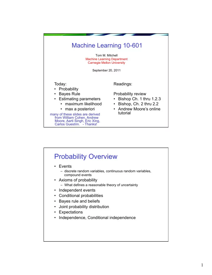
Machine Learning 10-601 Tom M. Mitchell Machine Learning Department Carnegie Mellon University September 20, 2011 Today: Readings: • Probability • Bayes Rule Probability review • Estimating parameters • Bishop Ch. 1 thru 1.2.3 • maximum likelihood • Bishop, Ch. 2 thru 2.2 • max a posteriori • Andrew Moore’s online tutorial many of these slides are derived from William Cohen, Andrew Moore, Aarti Singh, Eric Xing, Carlos Guestrin. - Thanks! Probability Overview • Events – discrete random variables, continuous random variables, compound events • Axioms of probability – What defines a reasonable theory of uncertainty • Independent events • Conditional probabilities • Bayes rule and beliefs • Joint probability distribution • Expectations • Independence, Conditional independence 1

Random Variables • Informally, A is a random variable if – A denotes something about which we are uncertain – perhaps the outcome of a randomized experiment • Examples A = True if a randomly drawn person from our class is female A = The hometown of a randomly drawn person from our class A = True if two randomly drawn persons from our class have same birthday • Define P(A) as “ the fraction of possible worlds in which A is true ” or “ the fraction of times A holds, in repeated runs of the random experiment ” – the set of possible worlds is called the sample space, S – A random variable A is a function defined over S A: S à {0,1} A little formalism More formally, we have • a sample space S (e.g., set of students in our class) – aka the set of possible worlds • a random variable is a function defined over the sample space – Gender: S à { m, f } – Height: S à Reals • an event is a subset of S – e.g., the subset of S for which Gender=f – e.g., the subset of S for which (Gender=m) AND (eyeColor=blue) • we’re often interested in probabilities of specific events • and of specific events conditioned on other specific events 2

Visualizing A Sample space of all possible P(A) = Area of Worlds in which worlds A is true reddish oval Worlds in which A is False Its area is 1 The Axioms of Probability • 0 <= P(A) <= 1 • P(True) = 1 • P(False) = 0 • P(A or B) = P(A) + P(B) - P(A and B) [di Finetti 1931]: when gambling based on “ uncertainty formalism A ” you can be exploited by an opponent iff your uncertainty formalism A violates these axioms 3

Interpreting the axioms • 0 <= P(A) <= 1 • P(True) = 1 • P(False) = 0 • P(A or B) = P(A) + P(B) - P(A and B) The area of A can ’ t get any smaller than 0 And a zero area would mean no world could ever have A true Interpreting the axioms • 0 <= P(A) <= 1 • P(True) = 1 • P(False) = 0 • P(A or B) = P(A) + P(B) - P(A and B) The area of A can ’ t get any bigger than 1 And an area of 1 would mean all worlds will have A true 4

Interpreting the axioms • 0 <= P(A) <= 1 • P(True) = 1 • P(False) = 0 • P(A or B) = P(A) + P(B) - P(A and B) Theorems from the Axioms • 0 <= P(A) <= 1, P(True) = 1, P(False) = 0 • P(A or B) = P(A) + P(B) - P(A and B) è P(not A) = P(~A) = 1-P(A) 5

Theorems from the Axioms • 0 <= P(A) <= 1, P(True) = 1, P(False) = 0 • P(A or B) = P(A) + P(B) - P(A and B) è P(not A) = P(~A) = 1-P(A) P(A or ~A) = 1 P(A and ~A) = 0 P(A or ~A) = P(A) + P(~A) - P(A and ~A) 1 = P(A) + P(~A) + 0 Elementary Probability in Pictures • P(~A) + P(A) = 1 A ~A 6

Another useful theorem • 0 <= P(A) <= 1, P(True) = 1, P(False) = 0, P(A or B) = P(A) + P(B) - P(A and B) è P(A) = P(A ^ B) + P(A ^ ~B) A = [A and (B or ~B)] = [(A and B) or (A and ~B)] P(A) = P(A and B) + P(A and ~B) – P((A and B) and (A and ~B)) P(A) = P(A and B) + P(A and ~B) – P(A and B and A and ~B) Elementary Probability in Pictures • P(A) = P(A ^ B) + P(A ^ ~B) A ^ B A ^ ~B B 7

Multivalued Discrete Random Variables • Suppose A can take on more than 2 values • A is a random variable with arity k if it can take on exactly one value out of {v 1 ,v 2 , ... v k } • Thus … P ( A v A v ) 0 if i j = ∧ = = ≠ i j P ( A = v 1 " A = v 2 " ... " A = v k ) = 1 Elementary Probability in Pictures k P ( A v ) 1 ∑ = = j j 1 = A=2 A=3 A=5 A=4 A=1 8

Definition of Conditional Probability P(A ^ B) P(A|B) = ----------- P(B) Corollary: The Chain Rule P(A ^ B) = P(A|B) P(B) Conditional Probability in Pictures picture: P(B|A=2) A=2 A=3 A=5 A=4 A=1 9

Independent Events • Definition: two events A and B are independent if Pr(A and B)=Pr(A)*Pr(B) • Intuition: knowing A tells us nothing about the value of B (and vice versa) Visualizing Probabilities A ^ B Sample space of all possible worlds A B Its area is 1 10

Definition of Conditional Probability P(A ^ B) P(A|B) = ----------- P(B) A B Definition of Conditional Probability P(A ^ B) P(A|B) = ----------- P(B) Corollary: The Chain Rule P(A ^ B) = P(A|B) P(B) P(C ^ A ^ B) = P(C|A ^ B) P(A|B) P(B) 11

Independent Events • Definition: two events A and B are independent if P(A ^ B)=P(A)*P(B) • Intuition: knowing A tells us nothing about the value of B (and vice versa) Bayes Rule • let’s write 2 expressions for P(A ^ B) A ^ B A B 12

P(B|A) * P(A) Bayes’ rule P(A|B) = P(B) we call P(A) the “prior” Bayes, Thomas (1763) An essay towards solving a problem in the doctrine and P(A|B) the “posterior” of chances. Philosophical Transactions of the Royal Society of London, 53:370-418 … by no means merely a curious speculation in the doctrine of chances, but necessary to be solved in order to a sure foundation for all our reasonings concerning past facts, and what is likely to be hereafter … . necessary to be considered by any that would give a clear account of the strength of analogical or inductive reasoning … Other Forms of Bayes Rule P ( B | A ) P ( A ) P ( A | B ) = P ( B | A ) P ( A ) P ( B |~ A ) P (~ A ) + P ( B | A X ) P ( A X ) ∧ ∧ P ( A | B X ) ∧ = P ( B X ) ∧ 13

Applying Bayes Rule P ( B | A ) P ( A ) P ( A | B ) = P ( B | A ) P ( A ) + P ( B |~ A ) P (~ A ) A = you have the flu, B = you just coughed Assume: P(A) = 0.05 P(B|A) = 0.80 P(B| ~A) = 0.2 what is P(flu | cough) = P(A|B)? what does all this have to do with function approximation? 14

The Joint Distribution Example: Boolean variables A, B, C A B C Prob Recipe for making a joint 0 0 0 0.30 distribution of M variables: 0 0 1 0.05 0 1 0 0.10 0 1 1 0.05 1 0 0 0.05 1 0 1 0.10 1 1 0 0.25 1 1 1 0.10 A 0.05 0.10 0.05 0.10 0.25 0.05 C 0.10 B 0.30 [A. Moore] The Joint Distribution Example: Boolean variables A, B, C A B C Prob Recipe for making a joint 0 0 0 0.30 distribution of M variables: 0 0 1 0.05 0 1 0 0.10 1. Make a truth table listing all 0 1 1 0.05 1 0 0 0.05 combinations of values of 1 0 1 0.10 your variables (if there are 1 1 0 0.25 M Boolean variables then 1 1 1 0.10 the table will have 2 M rows). A 0.05 0.10 0.05 0.10 0.25 0.05 C 0.10 B 0.30 [A. Moore] 15

The Joint Distribution Example: Boolean variables A, B, C A B C Prob Recipe for making a joint 0 0 0 0.30 distribution of M variables: 0 0 1 0.05 0 1 0 0.10 1. Make a truth table listing all 0 1 1 0.05 1 0 0 0.05 combinations of values of 1 0 1 0.10 your variables (if there are 1 1 0 0.25 M Boolean variables then 1 1 1 0.10 the table will have 2 M rows). 2. For each combination of A 0.05 0.10 0.05 values, say how probable it 0.10 is. 0.25 0.05 C 0.10 B 0.30 [A. Moore] The Joint Distribution Example: Boolean variables A, B, C A B C Prob Recipe for making a joint 0 0 0 0.30 distribution of M variables: 0 0 1 0.05 0 1 0 0.10 1. Make a truth table listing all 0 1 1 0.05 1 0 0 0.05 combinations of values of 1 0 1 0.10 your variables (if there are 1 1 0 0.25 M Boolean variables then 1 1 1 0.10 the table will have 2 M rows). 2. For each combination of A 0.05 0.10 0.05 values, say how probable it 0.10 is. 0.25 0.05 C 3. If you subscribe to the 0.10 axioms of probability, those B 0.30 numbers must sum to 1. [A. Moore] 16

Using the Joint One you have the JD P ( E ) P ( row ) ∑ = you can ask for the rows matching E probability of any logical expression involving your attribute [A. Moore] Using the Joint P(Poor Male) = 0.4654 P ( E ) P ( row ) ∑ = rows matching E [A. Moore] 17

Using the Joint P(Poor) = 0.7604 P ( E ) P ( row ) ∑ = rows matching E [A. Moore] Inference with the Joint P ( row ) ∑ P ( E E ) ∧ rows matching E and E P ( E | E ) 1 2 1 2 = = 1 2 P ( E ) P ( row ) ∑ 2 rows matching E 2 P(Male | Poor) = 0.4654 / 0.7604 = 0.612 [A. Moore] 18

Learning and the Joint Distribution Suppose we want to learn the function f: <G, H> à W Equivalently, P(W | G, H) Solution: learn joint distribution from data, calculate P(W | G, H) e.g., P(W=rich | G = female, H = 40.5- ) = [A. Moore] sounds like the solution to learning F: X à Y, or P(Y | X). Are we done? 19

[C. Guestrin] [C. Guestrin] 20

[C. Guestrin] Maximum Likelihood Estimate for Θ [C. Guestrin] 21

[C. Guestrin] [C. Guestrin] 22