a zoo of (discrete) Probability: Mean, Variance: random variables - - PowerPoint PPT Presentation

1

a zoo of (discrete) random variables

discrete uniform random variables A discrete random variable X equally likely to take any (integer) value between integers a and b, inclusive, is uniform. Notation: X ~ Unif(a,b) Probability: Mean, Variance:

2

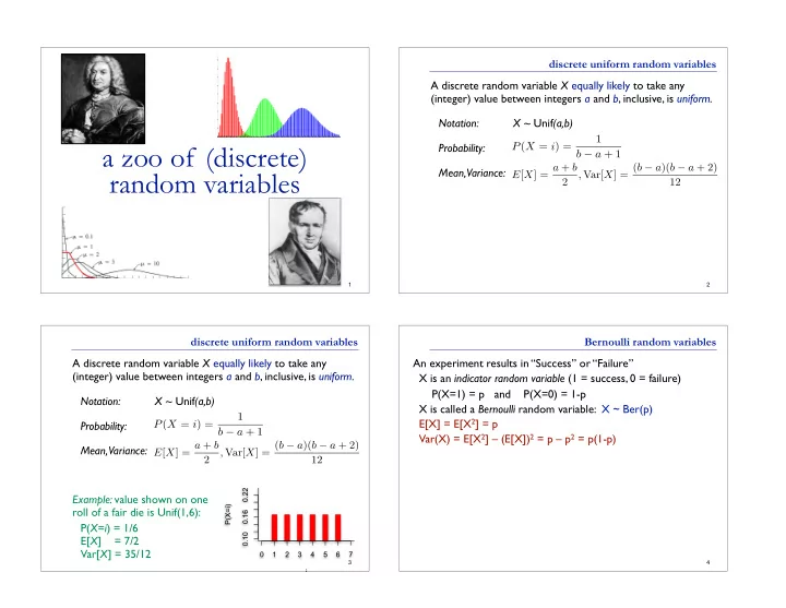
discrete uniform random variables A discrete random variable X equally likely to take any (integer) value between integers a and b, inclusive, is uniform. Notation: X ~ Unif(a,b) Probability: Mean, Variance: Example: value shown on one 
 roll of a fair die is Unif(1,6): P(X=i) = 1/6 
 E[X] = 7/2
 Var[X] = 35/12

3

1 2 3 4 5 6 7 0.10 0.16 0.22 i P(X=i)

Bernoulli random variables An experiment results in “Success” or “Failure” X is an indicator random variable (1 = success, 0 = failure) P(X=1) = p and P(X=0) = 1-p X is called a Bernoulli random variable: X ~ Ber(p) E[X] = E[X2] = p Var(X) = E[X2] – (E[X])2 = p – p2 = p(1-p)

4

Bernoulli random variables An experiment results in “Success” or “Failure” X is an indicator random variable (1 = success, 0 = failure) P(X=1) = p and P(X=0) = 1-p X is called a Bernoulli random variable: X ~ Ber(p) Examples: coin flip random binary digit whether a disk drive crashed

5

binomial random variables

Consider n independent random variables Yi ~ Ber(p) X = Σi Yi is the number of successes in n trials X is a Binomial random variable: X ~ Bin(n,p) Examples # of heads in n coin flips # of 1’s in a randomly generated length n bit string # of disk drive crashes in a 1000 computer cluster

6

binomial pmfs

7

2 4 6 8 10 0.00 0.05 0.10 0.15 0.20 0.25 0.30

PMF for X ~ Bin(10,0.5)

k P(X=k) µ ± σ 2 4 6 8 10 0.00 0.05 0.10 0.15 0.20 0.25 0.30

PMF for X ~ Bin(10,0.25)

k P(X=k) µ ± σ

binomial pmfs

8

5 10 15 20 25 30 0.00 0.05 0.10 0.15 0.20 0.25

PMF for X ~ Bin(30,0.5)

k P(X=k) µ ± σ 5 10 15 20 25 30 0.00 0.05 0.10 0.15 0.20 0.25

PMF for X ~ Bin(30,0.1)

k P(X=k) µ ± σ

mean, variance of the binomial (II)

9

In a series X1, X2, ... of Bernoulli trials with success probability p, let Y be the index of the first success, i.e., X1 = X2 = ... = XY-1 = 0 & XY = 1 Then Y is a geometric random variable with parameter p. geometric distribution

10

Examples: Number of coin flips until first head Number of blind guesses on SAT until I get one right Number of darts thrown until you hit a bullseye Number of random probes into hash table until empty slot Number of wild guesses at a password until you hit it In a series X1, X2, ... of Bernoulli trials with success probability p, let Y be the index of the first success, i.e., X1 = X2 = ... = XY-1 = 0 & XY = 1 Then Y is a geometric random variable with parameter p. P(Y=k) = (1-p)k-1p; Mean 1/p; Variance (1-p)/p2 geometric distribution

11

geometric distribution

12

Flip a (biased) coin repeatedly until 1st head observed How many flips? Let X be that number. P(X=1) = P(H) = p P(X=2) = P(TH) = (1-p)p P(X=3) = P(TTH) = (1-p)2p ... Check that it is a valid probability distribution: 1) 2)

memorize me!

Let X be the number of flips up to & including 1st head

• bserved in repeated flips of a biased coin.

A calculus trick: So (*) becomes: E.g.:

p=1/2; on average head every 2nd flip p=1/10; on average, head every 10th flip. P(H) = p; P(T) = 1 − p = q p(i) = pqi−1 E[X] = P

i≥1 ip(i) = P i≥1 ipqi−1 = p P i≥1 iqi−1

(∗)

13

geometric random variable Geo(p)

dy0/dy = 0

E[X] = p X

i≥1

iqi−1 = p (1 − q)2 = p p2 = 1 p

← PMF

models & reality Sending a bit string over the network n = 4 bits sent, each corrupted with probability 0.1 X = # of corrupted bits, X ~ Bin(4, 0.1) In real networks, large bit strings (length n ≈ 104) Corruption probability is very small: p ≈ 10-6 X ~ Bin(104, 10-6) is unwieldy to compute

Extreme n and p values arise in many cases

# bit errors in file written to disk 
 # of typos in a book # of elements in particular bucket of large hash table 
 # of server crashes per day in giant data center # facebook login requests sent to a particular server

14

Siméon Poisson, 1781-1840

Poisson random variables Suppose “events” happen, independently, at an average rate of λ per unit time. Let X be 
 the actual number of events happening in a given time unit. Then X is a Poisson r.v. with parameter λ (denoted X ~ Poi(λ)) and has distribution (PMF): Examples: # of alpha particles emitted by a lump of radium in 1 sec. # of traffic accidents in Seattle in one year # of babies born in a day at UW Med center # of visitors to my web page today

See B&T Section 6.2 for more on theoretical basis for Poisson.

15

poisson random variables

16

1 2 3 4 5 6 0.0 0.1 0.2 0.3 0.4 0.5 0.6 i P(X=i) λ = 0.5 λ = 3

X is a Poisson r.v. with parameter λ if it has PMF: Is it a valid distribution? Recall Taylor series: So poisson random variables

17

X is a Poisson r.v. with parameter λ if it has PMF: Is it a valid distribution? Recall Taylor series: So poisson random variables

18

expected value of poisson r.v.s

19

j = i-1

(Var[X] = λ, too; proof similar, see B&T example 6.20)

As expected, given definition in terms of “average rate λ” i = 0 term is zero

binomial —> Poisson in the limit

20

X ~ Binomial(n,p) Poisson approximates binomial when n is large, p is small, and λ = np is “moderate”

X ~ Binomial(n,p) I.e., Binomial ≈ Poisson for large n, small p, moderate i, λ.

Handy: Poisson has only 1 parameter–the expected # of successes

binomial → poisson in the limit

21

binomial random variable is poisson in the limit Poisson approximates binomial when n is large, p is small, and λ = np is “moderate” Different interpretations of “moderate,” e.g. n > 20 and p < 0.05 n > 100 and p < 0.1 Formally, Binomial is Poisson in the limit as 
 n → ∞ (equivalently, p → 0) while holding np = λ

22

sending data on a network Consider sending bit string over a network Send bit string of length n = 104 Probability of (independent) bit corruption is p = 10-6 X ~ Poi(λ = 104•10-6 = 0.01) What is probability that message arrives uncorrupted? Using Y ~ Bin(104, 10-6): P(Y=0) ≈ 0.990049829

I.e., Poisson approximation (here) is accurate to ~5 parts per billion

23 24

binomial vs poisson 2 4 6 8 10 0.00 0.10 0.20 k P(X=k) Binomial(10, 0.3) Binomial(100, 0.03) Poisson(3)

expectation and variance of a poisson Recall: if Y ~ Bin(n,p), then: E[Y] = pn Var[Y] = np(1-p) And if X ~ Poi(λ) where λ = np (n →∞, p → 0) then E[X] = λ = np = E[Y] Var[X] = λ ≈ λ(1-λ/n) = np(1-p) = Var[Y]

25

expectation and variance of a poisson Recall: if Y ~ Bin(n,p), then: E[Y] = pn Var[Y] = np(1-p) And if X ~ Poi(λ) where λ = np (n →∞, p → 0) then E[X] = λ = np = E[Y] Var[X] = λ ≈ λ(1-λ/n) = np(1-p) = Var[Y] Expectation and variance of Poisson are the same (λ) Expectation is the same as corresponding binomial Variance almost the same as corresponding binomial Note: when two different distributions share the same 
 mean & variance, it suggests (but doesn’t prove) that 


• ne may be a good approximation for the other.

26

balls in urns – the hypergeometric distribution Draw n balls (without replacement) from an urn containing N, of which m are white, the rest black. Let X = number of white balls drawn E[X] = np, where p = m/N (the fraction of white balls)

proof: Let Xj be 0/1 indicator for j-th ball is white, X = Σ Xj The Xj are dependent, but E[X] = E[Σ Xj] = Σ E[Xj] = np

Var[X] = np(1-p)(1-(n-1)/(N-1))

27

N

n

like binomial (almost)

P(X = i) = m

i

N−m

n−i

• N

n

• some important (discrete) distributions

28

Name PMF E[k] E[k2] σ2 Uniform(a, b) f(k) =

1 (b−a+1), k = a, a + 1, . . . , b a+b 2 (b−a+1)2−1 12

Bernoulli(p) f(k) =

(

1 − p if k = 0 p if k = 1 p p p(1 − p) Binomial(p, n) f(k) =

n

k

pk(1 − p)n−k, k = 0, 1, . . . , n

np np(1 − p) Poisson(λ) f(k) = e−λ λk

k! , k = 0, 1, . . .

λ λ(λ + 1) λ Geometric(p) f(k) = p(1 − p)k−1, k = 1, 2, . . .

1 p 2−p p2 1−p p2

Hypergeomet- ric(n, N, m) f(k) = (m

k)(N−m n−k )

(N

n)

, k = 0, 1, . . . , N

nm N nm N

⇣ (n−1)(m−1)

N−1

+ 1 − nm

N

⌘

E(X) E(X2)