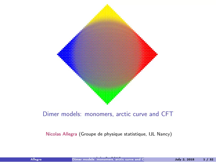
Dimer models: monomers, arctic curve and CFT Nicolas Allegra (Groupe - - PowerPoint PPT Presentation

Dimer models: monomers, arctic curve and CFT

Nicolas Allegra (Groupe de physique statistique, IJL Nancy) July 2, 2015

Allegra Dimer models: monomers, arctic curve and CFT July 2, 2015 1 / 32

1 Critical phenomena on rectangle geometry

Generalities about boundary conditions Critical free energy and CFT Correlation functions

2 Dimer models

Free boson theory Free fermion theory Corner free energy and exponents

3 Arctic circle phenomena and curved Dirac field

Arctic Circle Exact Calculations Asymptotic and field theory correspondence: toy model

4 Conclusions Allegra Dimer models: monomers, arctic curve and CFT July 2, 2015 2 / 32

Critical systems: Example of the Ising model

Free Free Free Free

Allegra Dimer models: monomers, arctic curve and CFT July 2, 2015 2 / 32

Critical systems: Example of the Ising model

Free Free Free Free

Some interesting questions

Change of boundary conditions → change of the critical behavior Expression of the free energy at the critical point Magnetization profile at the critical point Spin/energy correlation exponents close to a surface or corner

Allegra Dimer models: monomers, arctic curve and CFT July 2, 2015 2 / 32

Critical systems: Example of the Ising model

Free Free Free Free

Some interesting questions

Change of boundary conditions → change of the critical behavior Expression of the free energy at the critical point Magnetization profile at the critical point Spin/energy correlation exponents close to a surface or corner

Allegra Dimer models: monomers, arctic curve and CFT July 2, 2015 2 / 32

Ising model → c = 1/2 CFT

Free Free Free Free Free Free ++++

• - - -

Boundary condition changing operators (bcc)

(− − −) to (+ + +) or (Free) to (+ + +) or (− − −) to (Free) Ψ bcc primary operators of the c = 1/2 CFT Kac table c = 1/2 → hbcc = {0, 1/2, 1/16} Ψ+free = σ and Ψ+− = ϵ with h+free = 1/2 and h+− = 1/16 Boundary conformal field theory (Cardy ’84)

Allegra Dimer models: monomers, arctic curve and CFT July 2, 2015 3 / 32

Ising model → c = 1/2 CFT

Free Free Free Free Free Free ++++

• - - -

Boundary condition changing operators (bcc)

(− − −) to (+ + +) or (Free) to (+ + +) or (− − −) to (Free) Ψ bcc primary operators of the c = 1/2 CFT Kac table c = 1/2 → hbcc = {0, 1/2, 1/16} Ψ+free = σ and Ψ+− = ϵ with h+free = 1/2 and h+− = 1/16 Boundary conformal field theory (Cardy ’84)

Allegra Dimer models: monomers, arctic curve and CFT July 2, 2015 3 / 32

Ising model → c = 1/2 CFT

Free Free Free Free Free Free ++++

• - - -

Boundary condition changing operators (bcc)

(− − −) to (+ + +) or (Free) to (+ + +) or (− − −) to (Free) Ψ bcc primary operators of the c = 1/2 CFT Kac table c = 1/2 → hbcc = {0, 1/2, 1/16} Ψ+free = σ and Ψ+− = ϵ with h+free = 1/2 and h+− = 1/16 Boundary conformal field theory (Cardy ’84)

Allegra Dimer models: monomers, arctic curve and CFT July 2, 2015 3 / 32

Ising model → c = 1/2 CFT

Free Free Free Free Free Free ++++

• - - -

Boundary condition changing operators (bcc)

(− − −) to (+ + +) or (Free) to (+ + +) or (− − −) to (Free) Ψ bcc primary operators of the c = 1/2 CFT Kac table c = 1/2 → hbcc = {0, 1/2, 1/16} Ψ+free = σ and Ψ+− = ϵ with h+free = 1/2 and h+− = 1/16 Boundary conformal field theory (Cardy ’84)

Allegra Dimer models: monomers, arctic curve and CFT July 2, 2015 3 / 32

Ising model → c = 1/2 CFT

Free Free Free Free Free Free ++++

• - - -

Boundary condition changing operators (bcc)

(− − −) to (+ + +) or (Free) to (+ + +) or (− − −) to (Free) Ψ bcc primary operators of the c = 1/2 CFT Kac table c = 1/2 → hbcc = {0, 1/2, 1/16} Ψ+free = σ and Ψ+− = ϵ with h+free = 1/2 and h+− = 1/16 Boundary conformal field theory (Cardy ’84)

Allegra Dimer models: monomers, arctic curve and CFT July 2, 2015 3 / 32

Ising model → c = 1/2 CFT

Free Free Free Free Free Free ++++

• - - -

Boundary condition changing operators (bcc)

(− − −) to (+ + +) or (Free) to (+ + +) or (− − −) to (Free) Ψ bcc primary operators of the c = 1/2 CFT Kac table c = 1/2 → hbcc = {0, 1/2, 1/16} Ψ+free = σ and Ψ+− = ϵ with h+free = 1/2 and h+− = 1/16 Boundary conformal field theory (Cardy ’84)

Allegra Dimer models: monomers, arctic curve and CFT July 2, 2015 3 / 32

Free energy decomposition

F = L2fbulk + Lfsurface + fcorner fbulk and fsurface can be obtained by BA/TM but not fcorner

Corner free energy with a bcc operator

θ

¯ φb φb h

CFT predicts fcorner =

• π

θ hbcc + c 24

• θ

π − π θ

• log L universal (Cardy Peschel)

Valid close to criticality L → ξ Nice way to compute c and ξ (Vernier Jacobsen ’12)

Allegra Dimer models: monomers, arctic curve and CFT July 2, 2015 4 / 32

Free energy decomposition

F = L2fbulk + Lfsurface + fcorner fbulk and fsurface can be obtained by BA/TM but not fcorner

Corner free energy with a bcc operator

θ

¯ φb φb h

CFT predicts fcorner =

• π

θ hbcc + c 24

• θ

π − π θ

• log L universal (Cardy Peschel)

Valid close to criticality L → ξ Nice way to compute c and ξ (Vernier Jacobsen ’12)

Allegra Dimer models: monomers, arctic curve and CFT July 2, 2015 4 / 32

Free energy decomposition

F = L2fbulk + Lfsurface + fcorner fbulk and fsurface can be obtained by BA/TM but not fcorner

Corner free energy with a bcc operator

θ

¯ φb φb h

CFT predicts fcorner =

• π

θ hbcc + c 24

• θ

π − π θ

• log L universal (Cardy Peschel)

Valid close to criticality L → ξ Nice way to compute c and ξ (Vernier Jacobsen ’12)

Allegra Dimer models: monomers, arctic curve and CFT July 2, 2015 4 / 32

Free energy decomposition

F = L2fbulk + Lfsurface + fcorner fbulk and fsurface can be obtained by BA/TM but not fcorner

Corner free energy with a bcc operator

θ

¯ φb φb h

CFT predicts fcorner =

• π

θ hbcc + c 24

• θ

π − π θ

• log L universal (Cardy Peschel)

Valid close to criticality L → ξ Nice way to compute c and ξ (Vernier Jacobsen ’12)

Allegra Dimer models: monomers, arctic curve and CFT July 2, 2015 4 / 32

Bulk surface and corner correlations

• σ

b

( ) σ

b

( r )

• Correlations and scaling dimensions (spin σ and energy ϵ)

⟨σb(0)σb(r)⟩ ∼ r−xσ

b −xσ b

⟨ϵb(0)ϵb(r)⟩ ∼ r−xϵ

b−xϵ b

⟨σb(0)σs(r)⟩ ∼ r−xσ

b −xσ s

⟨ϵb(0)ϵs(r)⟩ ∼ r−xϵ

b−xϵ s

⟨σb(0)σc(r)⟩ ∼ r−xσ

b −xσ c

⟨ϵb(0)ϵc(r)⟩ ∼ r−xϵ

b−xϵ c

xb, xs, xc define bulk, surface and corner dimension of the operator xc and xs related by xc = (π/θ)xs Valid for all the primary operators of the CFT

Allegra Dimer models: monomers, arctic curve and CFT July 2, 2015 5 / 32

Bulk surface and corner correlations

• σ

b

( ) σ

b

( r )

• Correlations and scaling dimensions (spin σ and energy ϵ)

⟨σb(0)σb(r)⟩ ∼ r−xσ

b −xσ b

⟨ϵb(0)ϵb(r)⟩ ∼ r−xϵ

b−xϵ b

⟨σb(0)σs(r)⟩ ∼ r−xσ

b −xσ s

⟨ϵb(0)ϵs(r)⟩ ∼ r−xϵ

b−xϵ s

⟨σb(0)σc(r)⟩ ∼ r−xσ

b −xσ c

⟨ϵb(0)ϵc(r)⟩ ∼ r−xϵ

b−xϵ c

xb, xs, xc define bulk, surface and corner dimension of the operator xc and xs related by xc = (π/θ)xs Valid for all the primary operators of the CFT

Allegra Dimer models: monomers, arctic curve and CFT July 2, 2015 5 / 32

Bulk surface and corner correlations

• σ

b

( ) σ

b

( r )

• Correlations and scaling dimensions (spin σ and energy ϵ)

⟨σb(0)σb(r)⟩ ∼ r−xσ

b −xσ b

⟨ϵb(0)ϵb(r)⟩ ∼ r−xϵ

b−xϵ b

⟨σb(0)σs(r)⟩ ∼ r−xσ

b −xσ s

⟨ϵb(0)ϵs(r)⟩ ∼ r−xϵ

b−xϵ s

⟨σb(0)σc(r)⟩ ∼ r−xσ

b −xσ c

⟨ϵb(0)ϵc(r)⟩ ∼ r−xϵ

b−xϵ c

xb, xs, xc define bulk, surface and corner dimension of the operator xc and xs related by xc = (π/θ)xs Valid for all the primary operators of the CFT

Allegra Dimer models: monomers, arctic curve and CFT July 2, 2015 5 / 32

Bulk surface and corner correlations

• σ

b

( ) σ

b

( r )

• Correlations and scaling dimensions (spin σ and energy ϵ)

⟨σb(0)σb(r)⟩ ∼ r−xσ

b −xσ b

⟨ϵb(0)ϵb(r)⟩ ∼ r−xϵ

b−xϵ b

⟨σb(0)σs(r)⟩ ∼ r−xσ

b −xσ s

⟨ϵb(0)ϵs(r)⟩ ∼ r−xϵ

b−xϵ s

⟨σb(0)σc(r)⟩ ∼ r−xσ

b −xσ c

⟨ϵb(0)ϵc(r)⟩ ∼ r−xϵ

b−xϵ c

xb, xs, xc define bulk, surface and corner dimension of the operator xc and xs related by xc = (π/θ)xs Valid for all the primary operators of the CFT

Allegra Dimer models: monomers, arctic curve and CFT July 2, 2015 5 / 32

Bulk surface and corner correlations

• σ

b

( ) σ

b

( r )

• Correlations and scaling dimensions (spin σ and energy ϵ)

⟨σb(0)σb(r)⟩ ∼ r−xσ

b −xσ b

⟨ϵb(0)ϵb(r)⟩ ∼ r−xϵ

b−xϵ b

⟨σb(0)σs(r)⟩ ∼ r−xσ

b −xσ s

⟨ϵb(0)ϵs(r)⟩ ∼ r−xϵ

b−xϵ s

⟨σb(0)σc(r)⟩ ∼ r−xσ

b −xσ c

⟨ϵb(0)ϵc(r)⟩ ∼ r−xϵ

b−xϵ c

xb, xs, xc define bulk, surface and corner dimension of the operator xc and xs related by xc = (π/θ)xs Valid for all the primary operators of the CFT

Allegra Dimer models: monomers, arctic curve and CFT July 2, 2015 5 / 32

Definition of the model

Classical dimer model on the square lattice

η

H = − t 2

• ij

ηiAijηj, lattice considered. The nilp

Ising model with nilpotent variables (η2 = 0) instead of spins (σ2 = 1) Aij Connectivity (Adjacent) matrix Partition function

• Dη exp −H = √permA

Allegra Dimer models: monomers, arctic curve and CFT July 2, 2015 6 / 32

Combinatorial problem ↔ Physics problem

Selected chronology for dimer model on the square lattice (1937-2015)

Out[1130]=

Model of absorption of dimer molecules on a 2d substract (Fowler and Rushbrooke ’37) Partition function (Kasteleyn, Fisher and Temperley 1961) Solution by transfer matrix (Lieb ’67) Correlation functions dimer-dimer and monomer-monomer (Fisher Stephenson, Hartwig ’68) General correlation functions in terms of Ising correlations (Perk and Capel ’77) Solution by Grassmann variables (Hayn Plechko ’93) One monomer at the boundary by spanning tree mapping (Tzeng and Wu ’02) Arbitrary number of monomers at the boundary (Priezzhev Ruelle ’08) Arbitrary number of monomers anywhere (N.A and Fortin ’14) Other development: General monomer-dimer model (Heilmann and Lieb ’70, Baxter ’68) Quantum dimer model (Roshkar and Kivelson ’88). Interacting dimer model (Alet et Al ’05, Fradkin et Al ’06)...

Allegra Dimer models: monomers, arctic curve and CFT July 2, 2015 7 / 32

Kasteleyn pfaffian theory

Kasteleyn orientation

H = − t 2

• ij

aiKijaj Ising model with Grassmann variables (a2 = 0 and {ai, aj} = 0) Kij Kasteleyn (weighted Adjacent) matrix Partition function

• Da exp −H =

√ detK

Allegra Dimer models: monomers, arctic curve and CFT July 2, 2015 8 / 32

Kasteleyn modification for the monomer-dimer model

Modification of the orientation matrix K’ induced by monomers

Monomers on boundary → K’ is still a Kasteleyn Matrix Monomers creates changing-sign lines → K’ no more a Kasteleyn Matrix

Pfaffian perturbation theory (Fisher Stephenson 1963)

pf2(K ′) = pf2(K).det(1 + K −1E) where K ′ = K + E dimer-dimer correlation ⟨d(r)d(0)⟩ ∼ r−2 monomer-monomer correlation ⟨m(r)m(0)⟩ ∼ r−1/2

Allegra Dimer models: monomers, arctic curve and CFT July 2, 2015 9 / 32

Kasteleyn modification for the monomer-dimer model

Modification of the orientation matrix K’ induced by monomers

Monomers on boundary → K’ is still a Kasteleyn Matrix Monomers creates changing-sign lines → K’ no more a Kasteleyn Matrix

Pfaffian perturbation theory (Fisher Stephenson 1963)

pf2(K ′) = pf2(K).det(1 + K −1E) where K ′ = K + E dimer-dimer correlation ⟨d(r)d(0)⟩ ∼ r−2 monomer-monomer correlation ⟨m(r)m(0)⟩ ∼ r−1/2

Allegra Dimer models: monomers, arctic curve and CFT July 2, 2015 9 / 32

Kasteleyn modification for the monomer-dimer model

Modification of the orientation matrix K’ induced by monomers

Monomers on boundary → K’ is still a Kasteleyn Matrix Monomers creates changing-sign lines → K’ no more a Kasteleyn Matrix

Pfaffian perturbation theory (Fisher Stephenson 1963)

pf2(K ′) = pf2(K).det(1 + K −1E) where K ′ = K + E dimer-dimer correlation ⟨d(r)d(0)⟩ ∼ r−2 monomer-monomer correlation ⟨m(r)m(0)⟩ ∼ r−1/2

Allegra Dimer models: monomers, arctic curve and CFT July 2, 2015 9 / 32

Kasteleyn modification for the monomer-dimer model

Modification of the orientation matrix K’ induced by monomers

Monomers on boundary → K’ is still a Kasteleyn Matrix Monomers creates changing-sign lines → K’ no more a Kasteleyn Matrix

Pfaffian perturbation theory (Fisher Stephenson 1963)

pf2(K ′) = pf2(K).det(1 + K −1E) where K ′ = K + E dimer-dimer correlation ⟨d(r)d(0)⟩ ∼ r−2 monomer-monomer correlation ⟨m(r)m(0)⟩ ∼ r−1/2

Allegra Dimer models: monomers, arctic curve and CFT July 2, 2015 9 / 32

Grassmann variables and Berezin integration

Nilpotent and variables {η} and Grassmann variables {θ}

[ηi, ηj] = 0, η2

i = 0

• dη = 0
• dη.η = 1

{θi, θj} = 0, θ2

i = 0

• dθ = 0
• dθ.θ = 1

Berezin Integration over Grassmann variables {θi}

Berezin Integration: if f = f1 + θif2 then f2 =

∂f ∂θi and

• dθif (θi) = ∂f

∂θi Gaussian Integration det(A) =

α

dθαd¯ θα exp

αβ

θαAαβ ¯ θβ

• pf(A) =

α

dθα exp 1 2

• αβ

θαAαβθβ

• Allegra

Dimer models: monomers, arctic curve and CFT July 2, 2015 10 / 32

Grassmann variables and Berezin integration

Nilpotent and variables {η} and Grassmann variables {θ}

[ηi, ηj] = 0, η2

i = 0

• dη = 0
• dη.η = 1

{θi, θj} = 0, θ2

i = 0

• dθ = 0
• dθ.θ = 1

Berezin Integration over Grassmann variables {θi}

Berezin Integration: if f = f1 + θif2 then f2 =

∂f ∂θi and

• dθif (θi) = ∂f

∂θi Gaussian Integration det(A) =

α

dθαd¯ θα exp

αβ

θαAαβ ¯ θβ

• pf(A) =

α

dθα exp 1 2

• αβ

θαAαβθβ

• Allegra

Dimer models: monomers, arctic curve and CFT July 2, 2015 10 / 32

Grassmann formulation of the dimer model

Plechko partition function (using nilpotent variables)

η

→ Q0(L) =

• L
• m,n

dηmn(1 + txηmnηm+1n)(1 + tyηmnηmn+1)

Fermionization using Grassmann variables

η (a, ¯ a) (b,¯ b)

1 + txηmnηm+1n =

• d¯

amndamneamn¯

amn(1 + amnηmn)(1 + tx¯

amnηm+1n) = Tr{a,¯

a}Amn ¯

Am+1n 1 + tyηmnηmn+1 =

• d¯

bmndbmnebmn ¯

bmn(1 + bmnηmn)(1 + ty ¯

bmnηmn+1) = Tr{b,¯

b}Bmn ¯

Bmn+1

Allegra Dimer models: monomers, arctic curve and CFT July 2, 2015 11 / 32

Grassmann formulation of the dimer model

Plechko partition function (using nilpotent variables)

η

→ Q0(L) =

• L
• m,n

dηmn(1 + txηmnηm+1n)(1 + tyηmnηmn+1)

Fermionization using Grassmann variables

η (a, ¯ a) (b,¯ b)

1 + txηmnηm+1n =

• d¯

amndamneamn¯

amn(1 + amnηmn)(1 + tx¯

amnηm+1n) = Tr{a,¯

a}Amn ¯

Am+1n 1 + tyηmnηmn+1 =

• d¯

bmndbmnebmn ¯

bmn(1 + bmnηmn)(1 + ty ¯

bmnηmn+1) = Tr{b,¯

b}Bmn ¯

Bmn+1

Allegra Dimer models: monomers, arctic curve and CFT July 2, 2015 11 / 32

Grassmann formulation of the dimer model

Grassmann variables factorization

Associativity (O1 ¯ O2)(O2 ¯ O3)(O3 ¯ O4) = O1( ¯ O2O2)( ¯ O3O3) ¯ O4 Mirror ordering (O1 ¯ O1)(O2 ¯ O2)(O3 ¯ O3) = O1O2O3 ¯ O3 ¯ O2 ¯ O1

L

• m,n

(Amn ¯ Am+1n)(Bmn ¯ Bmn+1) = − →

• n=1

(A1n ¯ A2n)(B1n ¯ B1n+1)(A2n ¯ A3n)(B2n ¯ B2n+1) · · · = − →

• n=1

(A1n ¯ A2n)(A2n ¯ A3n) · · · (B1nB2n · · · ¯ B2n+1 ¯ B1n+1) = − →

• n=1

(B1n(A1n ¯ A2n)B2n(A2n ¯ A3n) · · · ¯ B2n+1 ¯ B1n+1) = − →

• n=1

(¯ BLn · · · ¯ B2n ¯ B1n)(B1nA1n ¯ A2nB2nA2n ¯ A3n · · · ¯ ALnBLnALn)

Mirror symmetry

Q0 = Tr{a,¯

a,b,¯ b,η}

− →

• n

← −

• m

¯ Bmn − →

• m

¯ AmnBmnAmn

• .

Allegra Dimer models: monomers, arctic curve and CFT July 2, 2015 12 / 32

Grassmann formulation of the dimer model

Grassmann variables factorization

Associativity (O1 ¯ O2)(O2 ¯ O3)(O3 ¯ O4) = O1( ¯ O2O2)( ¯ O3O3) ¯ O4 Mirror ordering (O1 ¯ O1)(O2 ¯ O2)(O3 ¯ O3) = O1O2O3 ¯ O3 ¯ O2 ¯ O1

L

• m,n

(Amn ¯ Am+1n)(Bmn ¯ Bmn+1) = − →

• n=1

(A1n ¯ A2n)(B1n ¯ B1n+1)(A2n ¯ A3n)(B2n ¯ B2n+1) · · · = − →

• n=1

(A1n ¯ A2n)(A2n ¯ A3n) · · · (B1nB2n · · · ¯ B2n+1 ¯ B1n+1) = − →

• n=1

(B1n(A1n ¯ A2n)B2n(A2n ¯ A3n) · · · ¯ B2n+1 ¯ B1n+1) = − →

• n=1

(¯ BLn · · · ¯ B2n ¯ B1n)(B1nA1n ¯ A2nB2nA2n ¯ A3n · · · ¯ ALnBLnALn)

Mirror symmetry

Q0 = Tr{a,¯

a,b,¯ b,η}

− →

• n

← −

• m

¯ Bmn − →

• m

¯ AmnBmnAmn

• .

Allegra Dimer models: monomers, arctic curve and CFT July 2, 2015 12 / 32

Solution and fermion field theory

Grassmann partition function

Q0 =

• D[a] D[¯

a] D[b] D[¯ b] − →

• m,n

Lmn[a, ¯ a, b, ¯ b] =

• D[a] D[¯

a] D[b] D[¯ b] D[c] exp

• mn

cmnLmn =

mn

dcmn exp

• mn

(txcmncm+1n + itycmncmn+1) =

• D[c] exp
• mn

S0[cmn] → Kasteleyn solution

Field theory → free fermions

S0[ψα, ψβ] = 1 2

• dxdy ψαMαβψβ

ψα,β Complex fermions ∈ even/odd sub-lattice such that ⟨ψαψα⟩ = ⟨ψβψβ⟩ = 0 ⟨ψα(0)ψβ(r)⟩ = M−1

αβ (r)

Allegra Dimer models: monomers, arctic curve and CFT July 2, 2015 13 / 32

Grassmann formulation with monomer

Modification of the partition function induced by monomers insertion

Q2n(L) =

• L
• m,n

dηmn(1 + txηmnηm+1n)(1 + tyηmnηmn+1)

• {ri }

ηmi ,ni Lmn → Lmn + hi Change of sign from ri to the boundary mi = L

Allegra Dimer models: monomers, arctic curve and CFT July 2, 2015 14 / 32

Partition function with monomers

Partition function of the dimer model with 2n monomers

Q2n =

• D[c] D[h] exp
• S0 +
• {ri }

cmi ni hi + 2ty

• {ri }

L

• m=mi +1

(−1)m+1cmni −1cmni

• .

”Free fermion” action S0 ”Grassmann Magnetic field” ”Topological defect line”

(m1, n1) (m4, n4) (m3, n3) (m2, n2)

Boundary

Pfaffian formulation

Q2n = pf(W )pf(C) W µν

αβ = δαβMµν α

+ V µν

αβ

→ W = dim(W ) = L2 × L2, dim(C) = 2n × 2n

Allegra Dimer models: monomers, arctic curve and CFT July 2, 2015 15 / 32

Partition function with monomers

Partition function of the dimer model with 2n monomers

Q2n =

• D[c] D[h] exp
• S0 +
• {ri }

cmi ni hi + 2ty

• {ri }

L

• m=mi +1

(−1)m+1cmni −1cmni

• .

”Free fermion” action S0 ”Grassmann Magnetic field” ”Topological defect line”

(m1, n1) (m4, n4) (m3, n3) (m2, n2)

Boundary

Pfaffian formulation

Q2n = pf(W )pf(C) W µν

αβ = δαβMµν α

+ V µν

αβ

→ W = dim(W ) = L2 × L2, dim(C) = 2n × 2n

Allegra Dimer models: monomers, arctic curve and CFT July 2, 2015 15 / 32

Boundary monomers → free fermion theory

Partition function of 2n boundary monomers and exact 2n-point correlations

If {ri} ∈ ∂B → W = M Q2n = Q0.pf(C) Q2n Q0 = ⟨c1c2...c2n⟩0 = pf(C) where |pf(C)| < 1 Exemple: 4-point correlations and Wick decomposition

Pf(C) = n1 n2 n3 n4 − + n1 n2 n3 n4 n1 n2 n3 n4

2-point function and Majorana Fermions

Cij = 4 [(−1)ni − (−1)nj ] (L + 1)2

L/2

• p,q=1

i1+ni +nj ty cos πq

L+1 sin2 πp L+1

t2

x cos2 πp L+1 + t2 y cos2 πq L+1

sin πqni L + 1 sin πqnj L + 1 Asymptotically ⟨cicj⟩0 ∼

−2 πdij if ni, nj /

∈ same sublattice 2 Complex chiral free fermions ⟨ψ(x)ψ†(y)⟩ = −

2 π(x−y) and ⟨ψ(x)ψ(y)⟩ = 0

Allegra Dimer models: monomers, arctic curve and CFT July 2, 2015 16 / 32

Boundary monomers → free fermion theory

Partition function of 2n boundary monomers and exact 2n-point correlations

If {ri} ∈ ∂B → W = M Q2n = Q0.pf(C) Q2n Q0 = ⟨c1c2...c2n⟩0 = pf(C) where |pf(C)| < 1 Exemple: 4-point correlations and Wick decomposition

Pf(C) = n1 n2 n3 n4 − + n1 n2 n3 n4 n1 n2 n3 n4

Cauchy determinant and superposition principle

Asymptotically Cij =

2 π|zi −wj | (zi/wi ∈ odd/even sublattice) then

• c1c2...cn
• 0 =

−2 π n det

• 1

zi − wj

• =
• i<j(zi − zj)

k<l(wk − wl)

• p<q(zp − wq)

Coulomb Gase: same/opposite sublattice = same/opposite charge

Cij ni nj Allegra Dimer models: monomers, arctic curve and CFT July 2, 2015 17 / 32

Bulk monomers = interacting theory

Partition function of 2n monomers and 2n-point correlations

If {ri} / ∈ ∂B → Q2nQ−1 = pf(WM−1).pf(C) = ⟨c1c2...c2n⟩I

⟨c1c2...c2n⟩I =

{ri }

ci exp

• 2ty

L

• m=mi +1

(−1)m+1cmni−1cmni

• Asymptotically ⟨ci cj ⟩I = Q(ri , rj )Q−1

∼ d−1/2

ij

(m1, n1) (m4, n4) (m3, n3) (m2, n2)

Boundary

Bulk vs surface criticality

bulk correlation ∼ r−1/2 surface correlation ∼ r−1 corner correlation ∼ r−1, r−2 or r−3

r−1/2 r−1 C(r) r

Allegra Dimer models: monomers, arctic curve and CFT July 2, 2015 18 / 32

Partition function with monomers

Partition function of the dimer model with 2n monomers

Q2n =

• D[c, h] exp
• S0 +
• {ri }

cmi ni hi + 2ty

• {ri }

L

• m=mi +1

(−1)m+1cmni −1cmni

• .

c = 1 Free fermion action S0 Grassmann Magnetic field Topological defect line

(m1, n1) (m4, n4) (m3, n3) (m2, n2)

Boundary

Pfaffian formulation

Q2n = pf(W )pf(C) W µν

αβ = δαβMµν α

+ V µν

αβ

→ W = dim(W ) = L2 × L2, dim(C) = 2n × 2n

Allegra Dimer models: monomers, arctic curve and CFT July 2, 2015 19 / 32

Partition function with monomers

Partition function of the dimer model with 2n monomers

Q2n =

• D[c, h] exp
• S0 +
• {ri }

cmi ni hi + 2ty

• {ri }

L

• m=mi +1

(−1)m+1cmni −1cmni

• .

c = 1 Free fermion action S0 Grassmann Magnetic field Topological defect line

(m1, n1) (m4, n4) (m3, n3) (m2, n2)

Boundary

Pfaffian formulation

Q2n = pf(W )pf(C) W µν

αβ = δαβMµν α

+ V µν

αβ

→ W = dim(W ) = L2 × L2, dim(C) = 2n × 2n

Allegra Dimer models: monomers, arctic curve and CFT July 2, 2015 19 / 32

Bosonic formulation of the dimer model

1 2 −1 −2 −1 −2 1 −3 1 1 −2 −1 −2 −1 2 −3 −4 −3 1 1 −2 −1 −2 −1 −2

c = 1 Free boson theory

Action: S[ϕ] = g

2

• dxdy
• ∇ϕ

2 where g stiffness Vertex operators: Ve,m(z) =: eieφ+imψ : where ∂iψ = ϵij∂jϕ Scaling dimensions: xg(e, m) =

e2 4πg + πgm2

Comparison with exact KFT results fixes g = 1/4π

1 1 1 −1 2 −1 −2 −1 −2 −1 1 −3 1 −1 −2 −1 −2 −1 2 −1 −3 −4 −3 1 −1 −2 −1 −2 −1 −2 −1 1 1 1

bcc operators

Change of boundary conditions in each corner hbcc =

g 2π ∆ϕ2 b = 1/32

Crucial for the extrapolation of the central charge Now we can look at the corner free energy !

Allegra Dimer models: monomers, arctic curve and CFT July 2, 2015 20 / 32

Bosonic formulation of the dimer model

1 2 −1 −2 −1 −2 1 −3 1 1 −2 −1 −2 −1 2 −3 −4 −3 1 1 −2 −1 −2 −1 −2

c = 1 Free boson theory

Action: S[ϕ] = g

2

• dxdy
• ∇ϕ

2 where g stiffness Vertex operators: Ve,m(z) =: eieφ+imψ : where ∂iψ = ϵij∂jϕ Scaling dimensions: xg(e, m) =

e2 4πg + πgm2

Comparison with exact KFT results fixes g = 1/4π

1 1 1 −1 2 −1 −2 −1 −2 −1 1 −3 1 −1 −2 −1 −2 −1 2 −1 −3 −4 −3 1 −1 −2 −1 −2 −1 −2 −1 1 1 1

bcc operators

Change of boundary conditions in each corner hbcc =

g 2π ∆ϕ2 b = 1/32

Crucial for the extrapolation of the central charge Now we can look at the corner free energy !

Allegra Dimer models: monomers, arctic curve and CFT July 2, 2015 20 / 32

Corner free energy and CFT

1 1 1 −1 2 −1 −2 −1 −2 −1 1 −3 1 −1 −2 −1 −2 −1 2 −1 −3 −4 −3 1 −1 −2 −1 −2 −1 −2 −1 1 1 1

Even size dimer model → Kasteleyn theory

Q0 = √ detK =

L

• p,q=1
• 4 cos2

πp L + 1 + 4 cos2 πq L + 1

• Asymptotic of Q0 gives fcorner = 0

4

• π

θ hbcc + c 24

• θ

π − π θ

• = 0 with 4 bcc operators with hbcc = 1/32 → c = 1

Allegra Dimer models: monomers, arctic curve and CFT July 2, 2015 21 / 32

Corner free energy and CFT

1 1 1 −1 2 −1 −2 −1 −2 −1 1 −3 1 −1 −2 −1 −2 −1 2 −1 −3 −4 −3 1 −1 −2 −1 −2 −1 −2 −1 1 1 1

Even size dimer model → Kasteleyn theory

Q0 = √ detK =

L

• p,q=1
• 4 cos2

πp L + 1 + 4 cos2 πq L + 1

• Asymptotic of Q0 gives fcorner = 0

4

• π

θ hbcc + c 24

• θ

π − π θ

• = 0 with 4 bcc operators with hbcc = 1/32 → c = 1

Allegra Dimer models: monomers, arctic curve and CFT July 2, 2015 21 / 32

Corner free energy and CFT

1 1 1 −1 2 −1 −2 −1 −2 −1 1 −3 1 −1 −2 −1 −2 −1 2 −1 −3 −4 −3 1 −1 −2 −1 −2 −1 −2 −1 1 1 1

Even size dimer model → Kasteleyn theory

Q0 = √ detK =

L

• p,q=1
• 4 cos2

πp L + 1 + 4 cos2 πq L + 1

• Asymptotic of Q0 gives fcorner = 0

4

• π

θ hbcc + c 24

• θ

π − π θ

• = 0 with 4 bcc operators with hbcc = 1/32 → c = 1

Allegra Dimer models: monomers, arctic curve and CFT July 2, 2015 21 / 32

Corner free energy and CFT

1 1 1 −1 2 −1 −2 −1 −2 −1 1 −3 1 −1 −2 −1 −2 −1 2 −1 −3 −4 −3 1 −1 −2 −1 −2 −1 −2 −1 1 1 1

Even size dimer model → Kasteleyn theory

Q0 = √ detK =

L

• p,q=1
• 4 cos2

πp L + 1 + 4 cos2 πq L + 1

• Asymptotic of Q0 gives fcorner = 0

4

• π

θ hbcc + c 24

• θ

π − π θ

• = 0 with 4 bcc operators with hbcc = 1/32 → c = 1

Allegra Dimer models: monomers, arctic curve and CFT July 2, 2015 21 / 32

Corner free energy and CFT 1 1 −2 3 −2

Odd size lattice with one monomer at the boundary (Tzeng-Wu)

Q1 =

L−1

• p,q=1
• 4 cos2

πp L + 1 + 4 cos2 πq L + 1

• Boundary monomers induce change of boundary conditions

Same analysis on a odd size lattice (with one monomer) gives fcorner = 1/2 log L Cardy Peschel formula with 3 bcc operators with hbcc = 1/32 and one with hbcc = 9/32 → c = 1

A similar analysis can be done in a c = −2 formalism !

Allegra Dimer models: monomers, arctic curve and CFT July 2, 2015 22 / 32

Corner free energy and CFT 1 1 −2 3 −2

Odd size lattice with one monomer at the boundary (Tzeng-Wu)

Q1 =

L−1

• p,q=1
• 4 cos2

πp L + 1 + 4 cos2 πq L + 1

• Boundary monomers induce change of boundary conditions

Same analysis on a odd size lattice (with one monomer) gives fcorner = 1/2 log L Cardy Peschel formula with 3 bcc operators with hbcc = 1/32 and one with hbcc = 9/32 → c = 1

A similar analysis can be done in a c = −2 formalism !

Allegra Dimer models: monomers, arctic curve and CFT July 2, 2015 22 / 32

Corner free energy and CFT 1 1 −2 3 −2

Odd size lattice with one monomer at the boundary (Tzeng-Wu)

Q1 =

L−1

• p,q=1
• 4 cos2

πp L + 1 + 4 cos2 πq L + 1

• Boundary monomers induce change of boundary conditions

Same analysis on a odd size lattice (with one monomer) gives fcorner = 1/2 log L Cardy Peschel formula with 3 bcc operators with hbcc = 1/32 and one with hbcc = 9/32 → c = 1

A similar analysis can be done in a c = −2 formalism !

Allegra Dimer models: monomers, arctic curve and CFT July 2, 2015 22 / 32

Corner free energy and CFT 1 1 −2 3 −2

Odd size lattice with one monomer at the boundary (Tzeng-Wu)

Q1 =

L−1

• p,q=1
• 4 cos2

πp L + 1 + 4 cos2 πq L + 1

• Boundary monomers induce change of boundary conditions

Same analysis on a odd size lattice (with one monomer) gives fcorner = 1/2 log L Cardy Peschel formula with 3 bcc operators with hbcc = 1/32 and one with hbcc = 9/32 → c = 1

A similar analysis can be done in a c = −2 formalism !

Allegra Dimer models: monomers, arctic curve and CFT July 2, 2015 22 / 32

Corner free energy and CFT 1 1 −2 3 −2

Odd size lattice with one monomer at the boundary (Tzeng-Wu)

Q1 =

L−1

• p,q=1
• 4 cos2

πp L + 1 + 4 cos2 πq L + 1

• Boundary monomers induce change of boundary conditions

Same analysis on a odd size lattice (with one monomer) gives fcorner = 1/2 log L Cardy Peschel formula with 3 bcc operators with hbcc = 1/32 and one with hbcc = 9/32 → c = 1

A similar analysis can be done in a c = −2 formalism !

Allegra Dimer models: monomers, arctic curve and CFT July 2, 2015 22 / 32

Critical exponents (bulk surface and corner)

Monomer and dimer scaling dimensions scaling dimension (gfree = 1/4π) bulk surface corner x(d) 1 1 2 x(m) 1/4 1/2 1/2 or 3/2

The monomer corner scaling dimension is not unique (Why ? IDK) In perfect agreement with the height mapping formulation Relation between corner and surface dimensions xc = π

θ xs satisfied

x(m,d)

b

x(m,d)

c

x(m,d)

s

Allegra Dimer models: monomers, arctic curve and CFT July 2, 2015 23 / 32

Dimer on the Aztec diamond

Aztec diamond dimer

Highly constrained configurations Highly excited boundaries → Non conformal boundaries Bipartite planar lattice → Kasteleyn still holds → free fermion S[ϕ] = g(x,y)

2

• dxdy
• ∇ϕ

2

2 3 2 4 5 4 5 4 6 6 7 7 6 3 6 8 9 8 5 8 5 4 5 8 6 7 6 7 6 3 6 4 5 4 5 4 2 3 2

Allegra Dimer models: monomers, arctic curve and CFT July 2, 2015 24 / 32

Arctic circle !!!

n

Main math results

Mapping to non-intersecting paths → Z = 2n(n+1)/2 (Why so simple ?) Gaussian fluctuations (bulk ∼ square lattice) Boundary fluctuations → corner growth process → GUE ensemble

Allegra Dimer models: monomers, arctic curve and CFT July 2, 2015 25 / 32

Arctic circle phenomenon in the dimer model

CFT

Disordered region

10 20 30 40 50 60

2d statistical problem → 1d quantum chain in imaginary time Transfer matrix T → Quantum hamiltonian H = − log T Particular initial and final state |ψ0⟩ → Domain wall initial state

Strategy

Step I → Compute fermion correlators exactly on the lattice Step II → Manage to study the scaling behavior (x/R and y/R fixed, R → ∞) Step III → Make a correspondance to correlators in a Dirac field theory

Allegra Dimer models: monomers, arctic curve and CFT July 2, 2015 26 / 32

Arctic circle phenomenon in the dimer model

CFT

Disordered region

10 20 30 40 50 60

2d statistical problem → 1d quantum chain in imaginary time Transfer matrix T → Quantum hamiltonian H = − log T Particular initial and final state |ψ0⟩ → Domain wall initial state

Strategy

Step I → Compute fermion correlators exactly on the lattice Step II → Manage to study the scaling behavior (x/R and y/R fixed, R → ∞) Step III → Make a correspondance to correlators in a Dirac field theory

Allegra Dimer models: monomers, arctic curve and CFT July 2, 2015 26 / 32

What kind of model can we tackle ?

Single band models (XX chain and hexagonal dimers)

H = dk 2π ε(k)c†(k)c(k) (1)

Two bands models (6-vertex and square dimers)

H = dk 2π ε+(k)a†(k)a(k) + ε−(k)b†(k)b(k) (2)

Allegra Dimer models: monomers, arctic curve and CFT July 2, 2015 27 / 32

Exact calculation on the lattice

Single Band expression

we are dealing with a free fermion problem, so every correlator can be reduced to a combination of two-point functions thanks to Wick’s theorem. Therefore, the quantity of interest is the propagator

• c†(x, y)c(x′, y′)
• ≡

        

⟨ψ|e−(R−y)H c†

x e−(y−y′)H cx′ e−(R+y′)H|ψ⟩

⟨ψ|e−2R H|ψ⟩

(y > y′) − ⟨ψ|e−(R−y′)H cx′ e−(y′−y)H c†

x e−(R+y)H|ψ⟩

⟨ψ|e−2R H|ψ⟩

(y < y′) going to momentum space, and using methods that are familiar from bosonization, one gets the key technical result

• c†(k, y)c(k′, y′)
• ≡ eiR(˜

ε(k)−˜ ε(k′)) e−(yε(k)−y′ε(k′))

2i sin

• k−k′

2

− i0+

• (3)

where ε(k) is the dispersion relation and ˜ ε(k) is its Hilbert transform, ˜ ε(k) ≡ p.v. π

−π

dk′ 2π ε(k′) cot k − k′ 2

• .

Allegra Dimer models: monomers, arctic curve and CFT July 2, 2015 28 / 32

1d electron gas in one slide

Hamiltonian in k space

H = dk 2π ε(k)c†(k)c(k) The low-energy theory is defined in terms of creation and annihilation operators in the vicinity of the Fermi points

Slow fields ψR and ψL

c(x) = √a(ψR(x, t)eikF x + ψL(x, t)e−ikF x) c†(x) = √a(ψ†

R(x, t)eikF x + ψ† L(x, t)e−ikF x)

such that {ψR(x, t), ψ†

R(x′, t)} = δ(x − x′)... etc

π kF vF EF

• kF

(R) ( L )

holes electrons

Λ

ψL and ψR → (1 + 1d) Dirac field theory L = i ¯ Ψ(γ0∂t − vγ1∂xΨ) with Ψ Dirac spinor with ψL and ψR component.

Allegra Dimer models: monomers, arctic curve and CFT July 2, 2015 29 / 32

1d electron gas in one slide

Hamiltonian in k space

H = dk 2π ε(k)c†(k)c(k) The low-energy theory is defined in terms of creation and annihilation operators in the vicinity of the Fermi points

Slow fields ψR and ψL

c(x) = √a(ψR(x, t)eikF x + ψL(x, t)e−ikF x) c†(x) = √a(ψ†

R(x, t)eikF x + ψ† L(x, t)e−ikF x)

such that {ψR(x, t), ψ†

R(x′, t)} = δ(x − x′)... etc

π kF vF EF

• kF

(R) ( L )

holes electrons

Λ

ψL and ψR → (1 + 1d) Dirac field theory L = i ¯ Ψ(γ0∂t − vγ1∂xΨ) with Ψ Dirac spinor with ψL and ψR component.

Allegra Dimer models: monomers, arctic curve and CFT July 2, 2015 29 / 32

Asymptotic analysis: General framework

Scaling regime (x/R and y/R fixed, R → ∞)

• c†(x, y)c(x′, y′)
• = e− 1

2 [σ(x,y)+σ(x′,y′)]

2πi   e−i[ϕ(x,y)−ϕ(x′,y′)] 2 sin

• z(x,y)−z(x′,y′)

2

− ei[ϕ∗(x,y)−ϕ∗(x′,y′)] 2 sin

• z∗(x,y)−z∗(x′,y′)

2

• 



Propagators of Dirac field Ψ† =

• ψ† ψ

†

• ψ†(x, y)ψ(x′, y′)
• = e− 1

2 [σ(x,y)+σ(x′,y′)]

e−i[ϕ(x,y)−ϕ(x′,y′)] 2 sin z(x,y)−z(x′,y′)

2

• + Gauge transformation Ψ(x, y) → ei Reϕ(x,y)γ5 e−Imϕ(x,y) Ψ(x, y) et

Ψ†(x, y) → Ψ†(x, y)e−i Reϕ(x,y)γ5 eImϕ(x,y) This is familiar to boundary CFT expert → correlators on a strip+non flat metric

Allegra Dimer models: monomers, arctic curve and CFT July 2, 2015 30 / 32

Asymptotic analysis: General framework

Scaling regime (x/R and y/R fixed, R → ∞)

• c†(x, y)c(x′, y′)
• = e− 1

2 [σ(x,y)+σ(x′,y′)]

2πi   e−i[ϕ(x,y)−ϕ(x′,y′)] 2 sin

• z(x,y)−z(x′,y′)

2

− ei[ϕ∗(x,y)−ϕ∗(x′,y′)] 2 sin

• z∗(x,y)−z∗(x′,y′)

2

• 



Propagators of Dirac field Ψ† =

• ψ† ψ

†

• ψ†(x, y)ψ(x′, y′)
• = e− 1

2 [σ(x,y)+σ(x′,y′)]

e−i[ϕ(x,y)−ϕ(x′,y′)] 2 sin z(x,y)−z(x′,y′)

2

• + Gauge transformation Ψ(x, y) → ei Reϕ(x,y)γ5 e−Imϕ(x,y) Ψ(x, y) et

Ψ†(x, y) → Ψ†(x, y)e−i Reϕ(x,y)γ5 eImϕ(x,y) This is familiar to boundary CFT expert → correlators on a strip+non flat metric

Allegra Dimer models: monomers, arctic curve and CFT July 2, 2015 30 / 32

Dirac action on a 2d curved metric

Curved Dirac field

S = 1 2π

• d2x
• det g eµ

a

i 2 Ψγa ↔ ∂µΨ

• .

(4) Here eµ

a is the tetrad, and (d2x

• det g) is the volume element. The spin connection drops out of

the two-dimensional Dirac action. We are free to chose the coordinate system, and it is natural to take the coordinates x1, x2 such that

• xz

= x1 + i x2 = z(x, y) x ¯

z

= x1 − i x2 = z∗(x, y) . In this coordinate system, we take the following tetrad: eµ

a = e−σδaµ ,

where σ is the function σ(x, y) that appeared previously; note that the metric is simply ds2 = e2σ (dx1)2 + (dx2)2 .

Exemple: Metric for the XX chain (dimer, 6vertex..much more complicated)

eσ(x,y) =

• R2 − x2 − y2

Allegra Dimer models: monomers, arctic curve and CFT July 2, 2015 31 / 32

Perspectives: In progress or not

Interesting questions

Connection with the bosonic theory ? Study of boundary correlations ? Explore the field theory more carefully, partition function ? Can we tell something interesting about the real time quench ? What remains true in the interacting case and what is wrong ?

Allegra Dimer models: monomers, arctic curve and CFT July 2, 2015 32 / 32