Differential Equations x i +1 x i x i +1 = x i + x x Physics-based - - PowerPoint PPT Presentation

Differential Equations

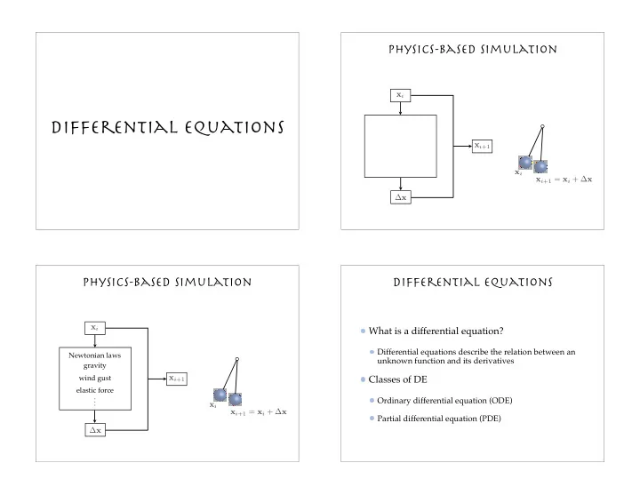
Physics-based simulation

xi ∆x xi+1 xi+1 = xi + ∆x xi

Physics-based simulation

xi ∆x xi+1 xi xi+1 = xi + ∆x

Newtonian laws gravity wind gust elastic force

. . .

Differential equations

What is a differential equation?

Differential equations describe the relation between an unknown function and its derivatives

Classes of DE

Ordinary differential equation (ODE) Partial differential equation (PDE)

Ordinary differential equations

An ODE is an equality involving a function and its derivatives What does it mean to “solve” an ODE? ˙ x(t) = f(x(t))

known function time derivative state of the system

Symbolic solutions

Standard introductory differential equation courses focus on finding solutions analytically Linear ODEs can be solved by integral transforms Use DSolve[eqn,x,t] in Mathematica

˙ x = −kx Differential equation: x = e−kt Solution:

Numerical solutions

• 3. increment x by to obtain new value

∆x

• 2. use this direction to approximate change over a

time interval ∆x ∆t

• 1. use f to calculate the derivative as the direction to next state

In this class, we will be concerned with numerical solutions Derivative function f is regarded as a black box: given numerical values for x and t, returns a numerical value for ˙ x

For each iteration:

Initial value problems

In a canonical initial value problem, the behavior of the system is described by an ODE and its initial condition: ˙ x = f(x, t) x(t0) = x0 To solve x(t) numerically, we start out from x0 and follow the changes defined by f thereafter

Vector field

How does the vector field look like if f depends directly on time?

The differential equation can be visualized as a vector field ˙ x = f(x, t)

x1 x2

p

Integral curves

Any point on the curve indicates the integral of from

f t0

t0 f(x, t) x

• t0

f(x, t)dt

Numerical methods

What do we know about the system? What are we trying to solve?

Get confused yet?

Numerical methods

Explicit methods

Explicit Euler’s method The midpoint method Runge-Kutta method

Implicit methods

Implicit Euler’s method

Explicit Euler ’s method

Discrete time step h determines the errors Instead of following real integral curve, p follows a polygonal path How do we get to the next state from the current state?

x(t0 + h) = x0 + h ˙ x(t0)

x(t0 + h) x(t0)

p

Problems of Euler ’s method

Inaccuracy The circle turns into a spiral no matter how small the step size is

Problems of Euler ’s method

Instability f = −kx

How small the step size has to be? Oscillation: Divergence:

Performance of Euler ’s method

x(t0 + h) = x(t0) + h ˙ x(t0) + h2 2! ¨ x(t0) + h3 3! x(3)(t0) + . . . hn n! ∂nx ∂tn

At each step, x(t) can be written in the form of Taylor series: What is the order of the error term in Euler’s method? Cost per step is determined by the number of evaluations per step

The midpoint method

• 2. Evaluate f at the midpoint
• 3. Take a step using fmid

fmid = f(x(t0) + ∆x 2 )

• 1. Compute an Euler’s step

∆x = hf(x(t0)) x(t0 + h) = x(t0) + hfmid x(t + h) = x0 + hf(x0 + h 2 f(x0))

Performance of midpoint method

Prove that the midpoint method is correct within O(h3)

Runge-Kutta method

Runge-Kutta is a numeric method of integrating ODEs by using a trial step at the midpoint of an interval to cancel out lower-order error terms The second order Runge-Kutta is known as the midpoint method q-stage p-order Runge-Kutta evaluates the derivative function q times in each iteration and its approximation

• f the next state is correct within O(hp+1)

4-stage 4th order Runge-Kutta

f(x0, t0) f(x0 + k1 2 , t0 + h 2 ) f(x0 + k2 2 , t0 + h 2 ) f(x0 + k3, t0 + h) x0 x(t0 + h) 2. 1. 3. 4.

k1 = hf(x0, t0) k2 = hf(x0 + k1

2 , t0 + h 2 )

k3 = hf(x0 + k2

2 , t0 + h 2 )

k4 = hf(x0 + k3, t0 + h) x(t0 + h) = x0 + 1

6k1 + 1 3k2 + 1 3k3 + 1 6k4

t x

Stage vs. order

p 1 2 3 4 5 6 7 8 9 10 qmin(p) 1 2 3 4 6 7 9 11 12-17 13-17

The minimum number of stages necessary for an explicit method to attain order p is still an open problem Why is fourth order the most popular Runge Kutta method?

Adaptive step size

Ideally, we want to choose h as large as possible, but not so large as to give us big error or instability We can vary h as we march forward in time

Step doubling Embedding estimate Variable step, variable order

Step doubling

e

xb = xtemp + h 2 f(xtemp, t0 + h 2 ) xtemp = x0 + h 2 f(x0, t0) Estimate by taking a full Euler step xa Estimate by taking two half Euler steps xb e = |xa − xb| is bound by O(h2) Given error tolerance , what is the optimal step size?

• e

1

2 h

xa = x0 + hf(x0, t0)

Embedding estimate

Also called Runge-Kutta-Fehlberg Compare two estimates of

Fifth order Runge-Kutta with 6 stages Forth order Runge-Kutta with 6 stages

x(t0 + h)

Variable step, variable order

Change between methods of different order as well as step based on obtained error estimates These methods are currently the last work in numerical integration

Problems of explicit methods

Do not work well with stiff ODEs

Simulation explodes if the step size is too big Simulation progresses slowly if the step size is too small

Example: a bead on the wire

˙ Y = d dt

• x(t)

y(t)

• =
• −x(t)

−ky(t)

• Y(t) = (x(t), y(t))

Ynew =

• (1 − h)x(t)

(1 − kh)y(t)

• Ynew = Y0 + h ˙

Y(t0) =

• x(t)

y(t)

• + h
• −x(t)

−ky(t)

• Explicit Euler’s method:

y(t) x(t)

Stiff equations

Stiffness constant: k Step size is limited by the largest k Systems that has some big k’s mixed in are called “stiff system”

Implicit methods

Implicit Euler:

Ynew = Y0 + hf(Ynew)

Explicit Euler:

Ynew = Y0 + hf(Y0)

Solving for such that , at time , points directly back at

• f

Ynew t0 + h Y0

Implicit method

Ynew = Y0 + hf(Y0) + h∆Yf (Y0) ∆Y = 1 hI − f (Y0) −1 f(Y0)

Approximating f(Ynew) by linearizing f(Y)

f(Ynew) = f(Y0) + ∆Yf (Y0) ∆Y = Ynew − Y0

, where Our goal is to solve for Ynew such that

Ynew = Y0 + hf(Ynew)

f(Y, t) = ˙ Y(t) f (Y, t) = ∂Y(t) ∂Y

Example: A bead on the wire

Apply the implicit Euler’s method to the bead-on-wire example

∆Y = 1 hI − f (Y0) −1 f(Y0)

= −1 −k

• f (Y(t)) = ∂f(Y(t))

∂Y f(Y(t)) = −x(t) −ky(t)

• ∆Y =
• 1+h

h 1+kh h

−1 −x0 −ky0

• =
• h

h+1 h 1+kh

−x0 −ky0

• = −
• h

h+1x0 h 1+khky0

• Example: A bead on the wire

What is the largest step size the implicit Euler’s method can take?

lim

h→∞ ∆Y = lim h→∞ −

• h

h+1x0 h 1+khky0

• = −
• x0

1 kky0

• = −
• x0

y0

• Ynew = Y0 + (−Y0) = 0

Implicit vs. explicit

explicit Euler: implicit Euler: correct solution: x(h) = e−hk x(h) = 1 1 + hk x(h) = 1 − hk

˙ x(h) = −kx(h) x(0) = 1 h x

Second-order implicit Euler

¨ x = f(x(t), ˙ x(t)) d dt

• x(t)

v(t)

• =
• v(t)

f(x, ˙ x)

• .

. .

• I − h∂f

∂v − h2 ∂f ∂x

• ∆v = h
• f(x0, ˙

x0) + h∂f ∂xv0

• Helpful hints

Don’t use explicit Euler’s method Do use adaptive step size

Modular implementation

Write solvers in terms of

Reusable solver code Simple model implementation

Generic operations:

Get dim(x) Get/Set x and t Derivative evaluation at current (x, t)

Solver interface

System Solver

GetDim Deriv Eval

Get/Set State

Summary

How do we solve an ODE numerically? What are the drawbacks of Explicit Euler’s method? What is a stiff system? Why does implicit Euler allow us to take bigger steps than explicit methods?

What’s next?

How do we use Euler’s method to simulate the motion of a mass point? What are the equations of motion when forces are applied to the mass point?