differential equations
play

Differential equations Programming of Differential Equations A - PowerPoint PPT Presentation

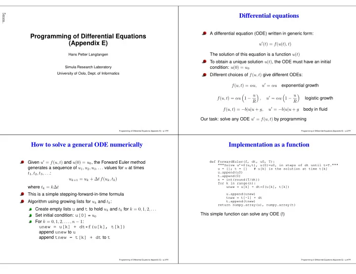
5mm. Differential equations Programming of Differential Equations A differential equation (ODE) written in generic form: (Appendix E) u ( t ) = f ( u ( t ) , t ) The solution of this equation is a function u ( t ) Hans Petter Langtangen To


  1. 5mm. Differential equations Programming of Differential Equations A differential equation (ODE) written in generic form: (Appendix E) u ′ ( t ) = f ( u ( t ) , t ) The solution of this equation is a function u ( t ) Hans Petter Langtangen To obtain a unique solution u ( t ) , the ODE must have an initial Simula Research Laboratory condition: u (0) = u 0 University of Oslo, Dept. of Informatics Different choices of f ( u, t ) give different ODEs: u ′ = αu f ( u, t ) = αu, exponential growth 1 − u 1 − u � � u ′ = αu � � f ( u, t ) = αu , logistic growth R R u ′ = − b | u | u + g f ( u, t ) = − b | u | u + g, body in fluid Our task: solve any ODE u ′ = f ( u, t ) by programming Programming of Differential Equations (Appendix E) – p.1/ ?? Programming of Differential Equations (Appendix E) – p.2/ ?? How to solve a general ODE numerically Implementation as a function Given u ′ = f ( u, t ) and u (0) = u 0 , the Forward Euler method def ForwardEuler(f, dt, u0, T): """Solve u’=f(u,t), u(0)=u0, in steps of dt until t=T.""" generates a sequence of u 1 , u 2 , u 3 , . . . values for u at times u = []; t = [] # u[k] is the solution at time t[k] u.append(u0) t 1 , t 2 , t 3 , . . . : t.append(0) u k +1 = u k + ∆ t f ( u k , t k ) n = int(round(T/dt)) for k in range(n): unew = u[k] + dt*f(u[k], t[k]) where t k = k ∆ t u.append(unew) This is a simple stepping-forward-in-time formula tnew = t[-1] + dt t.append(tnew) Algorithm using growing lists for u k and t k : return numpy.array(u), numpy.array(t) Create empty lists u and t to hold u k and t k for k = 0 , 1 , 2 , . . . Set initial condition: u[0] = u 0 This simple function can solve any ODE (!) For k = 0 , 1 , 2 , . . . , n − 1 : unew = u[k] + dt*f(u[k], t[k]) append unew to u append tnew = t[k] + dt to t Programming of Differential Equations (Appendix E) – p.3/ ?? Programming of Differential Equations (Appendix E) – p.4/ ??

  2. Example on using the function A class for solving ODEs Mathematical problem: Instead of a function for solving any ODE we now want to make a Solve u ′ = u , u (0) = 1 , for t ∈ [0 , 3] , with ∆ t = 0 . 1 class Basic code: Usage of the class: method = ForwardEuler(f, dt) def f(u, t): method.set_initial_condition(u0, t0) return u u, t = method.solve(T) u0 = 1 Store f , ∆ t , and the sequences u k , t k as attributes T = 3 dt = 0.1 Split the steps in the ForwardEuler function into three u, t = ForwardEuler(f, dt, u0, T) methods Compare exact and numerical solution: from scitools.std import plot, exp u_exact = exp(t) plot(t, u, ’r-’, t, u_exact, ’b-’, xlabel=’t’, ylabel=’u’, legend=(’numerical’, ’exact’), title="Solution of the ODE u’=u, u(0)=1") Programming of Differential Equations (Appendix E) – p.5/ ?? Programming of Differential Equations (Appendix E) – p.6/ ?? The code for a class for solving ODEs (part 1) The code for a class for solving ODEs (part 2) class ForwardEuler: class ForwardEuler: def __init__(self, f, dt): ... self.f, self.dt = f, dt def solve(self, T): """Advance solution in time until t <= T.""" def set_initial_condition(self, u0, t0=0): t = 0 self.u = [] # u[k] is solution at time t[k] while t < T: self.t = [] # time levels in the solution process unew = self.advance() # numerical formula self.u.append(unew) self.u.append(float(u0)) t = self.t[-1] + self.dt self.t.append(float(t0)) self.t.append(t) self.k = 0 # time level counter self.k += 1 return numpy.array(self.u), numpy.array(self.t) def advance(self): """Advance the solution one time step.""" # avoid "self." to get more readable formula: u, dt, f, k, t = \ self.u, self.dt, self.f, self.k, self.t[-1] unew = u[k] + dt*f(u[k], t) # Forward Euler scheme return unew Programming of Differential Equations (Appendix E) – p.7/ ?? Programming of Differential Equations (Appendix E) – p.8/ ??

  3. Using a class to hold the right-hand side f ( u, t ) Verifying the class implementation Mathematical problem: Mathematical problem: u ′ = 0 . 2 + ( u − h ( t )) 4 , � 1 − u ( t ) � u (0) = 3 , t ∈ [0 , 3] u ′ ( t ) = αu ( t ) , u (0) = u 0 , t ∈ [0 , 40] R u ( t ) = h ( t ) = 0 . 2 t + 3 (exact solution) Class for right-hand side f ( u, t ) : The Forward Euler method will reproduce such a linear u exactly! Code: class Logistic: def __init__(self, alpha, R, u0): self.alpha, self.R, self.u0 = alpha, float(R), u0 def f(u, t): return 0.2 + (u - h(t))**4 def __call__(self, u, t): # f(u,t) return self.alpha*u*(1 - u/self.R) def h(t): return 0.2*t + 3 Main program: u0 = 3; dt = 0.4; T = 3 method = ForwardEuler(f, dt) problem = Logistic(0.2, 1, 0.1) method.set_initial_condition(u0, 0) T = 40; dt = 0.1 u, t = method.solve(T) method = ForwardEuler(problem, dt) u_exact = h(t) method.set_initial_condition(problem.u0, 0) print ’Numerical: %s\nExact: %s’ % (u, u_exact) u, t = method.solve(T) Programming of Differential Equations (Appendix E) – p.9/ ?? Programming of Differential Equations (Appendix E) – p.10/ ?? Figure of the solution Ordinary differential equations Mathematical problem: Logistic growth: alpha=0.2, dt=0.1, 400 steps 1 u ′ ( t ) = f ( u, t ) 0.9 Initial condition: 0.8 u (0) = u 0 0.7 Possible applications: 0.6 u 0.5 Exponential growth of money or populations: f ( u, t ) = αu , α = const 0.4 Logistic growth of a population under limited resources: 0.3 0.2 1 − u � � f ( u, t ) = αu R 0.1 0 5 10 15 20 25 30 35 40 t where R is the maximum possible value of u Radioactive decay of a substance: f ( u, t ) = − αu , α = const Programming of Differential Equations (Appendix E) – p.11/ ?? Programming of Differential Equations (Appendix E) – p.12/ ??

  4. Numerical solution of ordinary differential equations A superclass for ODE methods Numerous methods for u ′ ( t ) = f ( u, t ) , u (0) = u 0 Common tasks for ODE solvers: The Forward Euler method: Store the solution u k and the corresponding time levels t k , k = 0 , 1 , 2 , . . . , N u k +1 = u k + ∆ t f ( u k , t k ) Store the right-hand side function f ( u, t ) The 4th-order Runge-Kutta method: Store the time step ∆ t and last time step number k Set the initial condition u k +1 = u k + 1 6 ( K 1 + 2 K 2 + 2 K 3 + K 4 ) Implement the loop over all time steps Code for the steps above are common to all classes and hence placed in superclass ODESolver = ∆ t f ( u k , t k ) , K 1 ∆ t f ( u k + 1 2 K 1 , t k + 1 Subclasses, e.g., ForwardEuler , just implement the specific K 2 = 2∆ t ) , stepping formula in a method advance ∆ t f ( u k + 1 2 K 2 , t k + 1 K 3 = 2∆ t ) , K 4 = ∆ t f ( u k + K 3 , t k + ∆ t ) There is a jungle of different methods – how to program? Programming of Differential Equations (Appendix E) – p.13/ ?? Programming of Differential Equations (Appendix E) – p.14/ ?? The superclass code Implementation of the Forward Euler method class ODESolver: Subclass code: def __init__(self, f, dt): self.f = f class ForwardEuler(ODESolver): self.dt = dt def advance(self): u, dt, f, k, t = \ def set_initial_condition(self, u0, t0=0): self.u, self.dt, self.f, self.k, self.t[-1] self.u = [] # u[k] is solution at time t[k] self.t = [] # time levels in the solution process unew = u[k] + dt*f(u[k], t) self.u.append(u0) return unew self.t.append(t0) self.k = 0 # time level counter Application code for u ′ = u , u (0) = 1 , t ∈ [0 , 3] , ∆ t = 0 . 1 : def solve(self, T): t = 0 from ODESolver import ForwardEuler while t < T: def test1(u, t): unew = self.advance() # the numerical formula return u self.u.append(unew) method = ForwardEuler(test1, dt=0.1) t = self.t[-1] + self.dt method.set_initial_condition(u0=1) self.t.append(t) u, t = method.solve(T=3) self.k += 1 plot(t, u) return numpy.array(self.u), numpy.array(self.t) def advance(self): raise NotImplementedError Programming of Differential Equations (Appendix E) – p.15/ ?? Programming of Differential Equations (Appendix E) – p.16/ ??

Download Presentation
Download Policy: The content available on the website is offered to you 'AS IS' for your personal information and use only. It cannot be commercialized, licensed, or distributed on other websites without prior consent from the author. To download a presentation, simply click this link. If you encounter any difficulties during the download process, it's possible that the publisher has removed the file from their server.

Recommend


More recommend