CS411 balanced search tree Database Systems hash table R etc - - PDF document

CS411 Database Systems

Kazuhiro Minami 12: Query Optimization

One-pass Algorithms

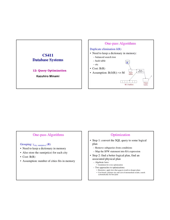
Duplicate elimination δ(R)

• Need to keep a dictionary in memory:

– balanced search tree – hash table – etc

• Cost: B(R)
• Assumption: B(δ(R)) <= M

R

Input buffer Scan before?

M-1 buffers

Output buffer

One-pass Algorithms

Grouping: γcity, sum(price) (R)

• Need to keep a dictionary in memory
• Also store the sum(price) for each city
• Cost: B(R)
• Assumption: number of cities fits in memory

Optimization

• Step 1: convert the SQL query to some logical

plan

– Remove subqueries from conditions – Map the SFW statement into RA expression

• Step 2: find a better logical plan, find an

associated physical plan

– Algebraic laws:

• foundation for every optimization

– Two approaches to optimizations:

• Heuristics: apply laws that seem to result in cheaper plans
• Cost based: estimate size and cost of intermediate results, search

systematically for best plan

SQL –> Logical Query Plans Converting from SQL to Logical Plans

Select a1, …, an From R1, …, Rk Where C Select a1, …, an From R1, …, Rk Where C

Πa1,…,an(σ C(R1 × R2 × … × Rk)) Πa1,…,an(γ b1, …, bm, aggs (σ C(R1 × R2 × … × Rk)))

Select a1, …, an From R1, …, Rk Where C Group by b1, …, bl Select a1, …, an From R1, …, Rk Where C Group by b1, …, bl

Some nested queries can be flattened

Select distinct product.name From product Where product.maker in (Select company.name From company where company.city=“Urbana”) Select distinct product.name From product Where product.maker in (Select company.name From company where company.city=“Urbana”)

Select distinct product.name From product, company Where product.maker = company.name AND company.city=“Urbana” Select distinct product.name From product, company Where product.maker = company.name AND company.city=“Urbana”

Converting Nested Queries

Select distinct x.name, x.maker From product x Where x.color= “blue” AND x.price >= ALL (Select y.price From product y Where x.maker = y.maker AND y.color=“blue”) Select distinct x.name, x.maker From product x Where x.color= “blue” AND x.price >= ALL (Select y.price From product y Where x.maker = y.maker AND y.color=“blue”)

Q: How do we convert this one to logical plan ?

Q: Give a list of product-manufacture pairs where the color of the product is blue and its prices is the highest among the products with blue color from that manufacture.

Converting Nested Queries

Select distinct x.name, x.maker From product x Where x.color= “blue” AND x.price < SOME (Select y.price From product y Where x.maker = y.maker AND y.color=“blue”) Select distinct x.name, x.maker From product x Where x.color= “blue” AND x.price < SOME (Select y.price From product y Where x.maker = y.maker AND y.color=“blue”)

Let’s compute the complement first:

Converting Nested Queries

Select distinct x.name, x.maker From product x, product y Where x.color= “blue” AND x.maker = y.maker AND y.color=“blue” AND x.price < y.price Select distinct x.name, x.maker From product x, product y Where x.color= “blue” AND x.maker = y.maker AND y.color=“blue” AND x.price < y.price This one becomes a query without subqueries: This returns exactly the products we DON’T want, so…

A set difference operator finishes the job

(Select x.name, x.maker From product x Where x.color = “blue”) EXCEPT (Select x.name, x.maker From product x, product y Where x.color= “blue” AND x.maker = y.maker AND y.color=“blue” AND x.price < y.price) (Select x.name, x.maker From product x Where x.color = “blue”) EXCEPT (Select x.name, x.maker From product x, product y Where x.color= “blue” AND x.maker = y.maker AND y.color=“blue” AND x.price < y.price)

Now rewrite the logical plan to an equivalent but better one

Same query answer

Optimizer uses algebraic laws Equivalen t Original

Will probably run faster

Cost-based:

estimate size and cost

• f intermediate results,

search systematically for best plan

Heuristic:

likely to result in cheaper plans

Algebraic Laws Algebraic Laws

• Commutative and Associative Laws

– R ∪ S = S ∪ R, R ∪ (S ∪ T) = (R ∪ S) ∪ T – R ∩ S = S ∩ R, R ∩ (S ∩ T) = (R ∩ S) ∩ T – R ⋈ S = S ⋈ R, R ⋈ (S ⋈ T) = (R ⋈ S) ⋈ T

• Distributive Laws

– R ⋈ (S ∪ T) = (R ⋈ S) ∪ (R ⋈ T)

Algebraic laws about selections

σC AND D (R) = σC (σD (R)) = σC (R) ∩ σD (R) σC OR D (R) = σC (R) ∪ σD (R) σC (R ∪ S) = σC (R) ∪ σC (S) σC (R ⋈ S) = σC (R) ⋈ S σC (R – S) = σC (R) – S σC (R ∩ S) = σC (R) ∩ S

i i f f C C i n i n v v

• l

l v v e e s s

• n

n l y l y a a t t t t r r i b i b u u t t e e s s

• f

f R R

R(A,B,C,D) S(E,F,G)

σ F=3 (R ⋈D=E S) = σ A=5 AND G=9 (R ⋈D=E S) =

(R ⋈D=E σ F=3 (S)) σA=5 (σ G=9(R ⋈D=E S)) = σA=5 (R ⋈D=E σG=9 (S)) = σA=5 (R) ⋈D=E σG=9 (S)

Algebraic laws for projection

ΠM(R ⋈ S) = ΠN(ΠP(R) ⋈ ΠQ(S))

where N, P, Q are appropriate subsets of attributes of M

ΠM(ΠN(R)) = ΠM,N(R)

R(A,B,C,D) S(E,F,G)

ΠA,B,G(R ⋈D=E S) = Π ? (Π?(R) ⋈D=E Π?(S))

Algebraic laws for grouping and aggregation

δ (γA, agg(B)(R)) = γA, agg(B)(R) γA, agg(B)(δ(R)) = γA, agg(B)(R),

if agg is duplicate insensitive

The book describes additional algebraic laws, but even the book doesn’t cover them all.

SUM COUNT AVG MIN MAX

Heuristics-based Optimization

• or –

Do projections and selections as early as possible Heuristic Based Optimizations

• Query rewriting based on algebraic laws
• Result in better queries most of the time
• Heuristics number 1:

– Push selections down

• Heuristics number 2:

– Sometimes push selections up, then down

Predicate Pushdown

Product Company

maker=name

σ price>100 AND city=“Urbana”

pname

Product Company

maker=name price>100 pname city=“Urbana”

(but may cause us to lose an important ordering

• f the tuples, if we use indexes).

For each company with a product costing more than $100, find the max price of its products

Select y.name, y.address, Max(x.price) From product x, company y Where x.maker = y.name GroupBy y.name Having Max(x.price) > 100 Select y.name, y.address, Max(x.price) From product x, company y Where x.maker = y.name GroupBy y.name Having Max(x.price) > 100 Select y.name, y.address, Max(x.price) From product x, company y Where x.maker=y.name and x.price > 100 GroupBy y.name Having Max(x.price) > 100 Select y.name, y.address, Max(x.price) From product x, company y Where x.maker=y.name and x.price > 100 GroupBy y.name Having Max(x.price) > 100

• Advantage: the size of the join will be smaller.
• Requires transformation rules specific to the grouping/aggregation
• perators.
• Won’t work if we replace Max by Min.

Pushing predicates up

Create View V1 AS Select x.category, Min(x.price) AS p From product x Where x.price < 20 GroupBy x.category Create View V1 AS Select x.category, Min(x.price) AS p From product x Where x.price < 20 GroupBy x.category Create View V2 AS Select y.cname, x.category, x.price From product x, company y Where x.maker=y.cname Create View V2 AS Select y.cname, x.category, x.price From product x, company y Where x.maker=y.cname Select V2.category, V2.cname, V2.price From V1, V2 Where V1.category = V2.category and V1.p = V2.price Select V2.category, V2.cname, V2.price From V1, V2 Where V1.category = V2.category and V1.p = V2.price

V1: categories and the cheapest price of the product in that category under $20 V2: Company name, product category, and the price of the product made by that company

Query Rewrite: Pushing predicates up

Create View V1 AS Select x.category, Min(x.price) AS p From product x Where x.price < 20 GroupBy x.category Create View V1 AS Select x.category, Min(x.price) AS p From product x Where x.price < 20 GroupBy x.category Create View V2 AS Select y.cname, x.category, x.price From product x, company y Where x.maker=y.cname Create View V2 AS Select y.cname, x.category, x.price From product x, company y Where x.maker=y.cname Select V2.cname, V2.price From V1, V2 Where V1.category = V2.category and V1.p = V2.price AND V1.p < 20 Select V2.cname, V2.price From V1, V2 Where V1.category = V2.category and V1.p = V2.price AND V1.p < 20

25

Query Rewrite: Pushing predicates up

Create View V1 AS Select x.category, Min(x.price) AS p From product x Where x.price < 20 GroupBy x.category Create View V1 AS Select x.category, Min(x.price) AS p From product x Where x.price < 20 GroupBy x.category Create View V2 AS Select y.cname, x.category, x.price From product x, company y Where x.maker=y.cname AND x.price < 20 Create View V2 AS Select y.cname, x.category, x.price From product x, company y Where x.maker=y.cname AND x.price < 20 Select V2.cname, V2.price From V1, V2 Where V1.category = V2.category and V1.p = V2.price AND V1.p < 20 Select V2.cname, V2.price From V1, V2 Where V1.category = V2.category and V1.p = V2.price AND V1.p < 20

Cost-based Optimization Cost-based Optimizations

• Main idea: apply algebraic laws, until estimated

cost is minimal

• Practically: start from partial plans, introduce
• perators one by one

– Will see in a few slides

• Problem: there are too many ways to apply the

laws, hence too many (partial) plans

Often: generate a partial plan, optimize it, then add another operator, …

Top-down: the partial plan is a top fragment of the logical plan Bottom up: the partial plan is a bottom fragment of the logical plan

Search Strategies

• Branch-and-bound:

– Remember the cheapest complete plan P seen by using heuristics so far and its cost C – Stop generating partial plans whose cost is > C – If a cheaper complete plan P is found, replace C with P

• Hill climbing:

– Find nearby plans that have lower cost by making small changes to the plan

• Dynamic programming:

– Compute cheapest partial plans of the smallest and compute cheapest partial plans of larger size next – Remember the all cheapest partial plans

Algebraic Laws for Joins

• Commutative and Associative Laws

– R ∪ S = S ∪ R, R ∪ (S ∪ T) = (R ∪ S) ∪ T – R ∩ S = S ∩ R, R ∩ (S ∩ T) = (R ∩ S) ∩ T – R ⋈ S = S ⋈ R, R ⋈ (S ⋈ T) = (R ⋈ S) ⋈ T

• Distributive Laws

– R ⋈ (S ∪ T) = (R ⋈ S) ∪ (R ⋈ T)

The order that relations are joined in has a huge impact on performance

Given: query R1 ⋈ … ⋈ Rn, function cost( ), find the best join tree for the query

R3 R1 R2 R4 Pl Plan = tree Partia ial p l plan = subtree

Types of Join Trees

• Left deep (all right children are leaves)

R3 R1 R5 R2 R4

Types of Join Trees

• Right deep (all left children are leaves)

R3 R1 R5 R2 R4

Types of Join Trees

• Bushy if neither left-deep nor right-deep

R3 R1 R2 R4 R5

Dynamic programming is a good (bottom-up) way to choose join ordering

Find the best plan for each subquery Q of {R1, …, Rn}:

• 1. {R1}, …, {Rn}
• 2. {R1, R2}, {R1, R3}, …,

{Rn-1, Rn}

• 3. {R1, R2, R3}, {R1, R2, R4},

…

• 4. …
• 5. {R1, …, Rn}

Output:

• 1. Size(Q)
• 2. A best plan

Plan(Q)

• 3. Cost(Q)

The ith step of the dynamic program

For each Q ⊆ {R1, …, Rn} of size i do:

• 1. Compute Size(Q)

(later…)

• 2. For every pair Q1, Q2 such that Q = Q1 ∪ Q2,

compute cost(Plan(Q1) ⋈ Plan(Q2)) Cost(Q) = the smallest such cost Plan(Q) = the corresponding plan

Dynamic Programming

• Return Plan({R1, …, Rn})

Dynamic Programming

To illustrate, we will make the following simplifications:

• Cost(P1 ⋈ P2) = Cost(P1) + Cost(P2) +

size(intermediate results for P1 and P2)

• Intermediate results:

– If P1 is a join, then the size of the intermediate result is size(P1), otherwise the size is 0 – Similarly for P2

• Cost of a scan = 0

Dynamic Programming

• Example:
• Cost(R5 ⋈ R7)

= Cost(R5) + Cost(R7) + intermediate results for R5 and R7 = 0 (no intermediate results)

• Cost((R2 ⋈ R1) ⋈ R7)

= Cost(R2 ⋈ R1) + Cost(R7) + size(R2 ⋈ R1) = size(R2 ⋈ R1)

Dynamic Programming

• Relations: R, S, T, U
• Number of tuples: 2000, 5000, 3000, 1000
• Size estimation: T(A ⋈ B) = 0.01*T(A)*T(B)

Subquery Size Cost Plan RS RT RU ST SU TU RST RSU RTU STU RSTU

T(R) = 2000 T(S) = 5000 T(T) = 3000 T(U) = 1000

T(A ⋈ B) = 0.01*T(A)*T(B) 100k RS 60K 0 RT 20K 0 RU 150K 0 ST 50K 0 SU 30K 0 TU

0.01 * T(R) * T(S) = 0.01 * 2000 * 5000 = 100,000 = 100k

Subquery Size Cost Plan RS RT RU ST SU TU RST RSU RTU STU RSTU

T(R) = 2000 T(S) = 5000 T(T) = 3000 T(U) = 1000 T(A ⋈ B) = 0.01*T(A)*T(B)

100K RS 60K 0 RT 20K 0 RU 150K 0 ST 50K 0 SU 30K 0 TU Cost((RS)T) = Cost((RS)T) = Cost(RS) + Cost(T) + size(RS) = 100k Cost((RT)S) = Cost((RT)S) = Cost(RT) + Cost(S) + size(RT) = 60k Cost((ST)R) = 150k 3M 60K (RT)S 1M 20K (RU)S 0.6M 20K (RU)T 1.5M 30K (TU)S

Subquery Size Cost Plan RS RT RU ST SU TU RST RSU RTU STU RSTU

T(R) = 2000 T(S) = 5000 T(T) = 3000 T(U) = 1000 T(A ⋈ B) = 0.01*T(A)*T(B)

100K RS 60K 0 RT 20K 0 RU 150K 0 ST 50K 0 SU 30K 0 TU 3M 60K (RT)S 1M 20K (RU)S 0.6M 20K (RU)T 1.5M 30K (TU)S

1. Cost(R(STU)) = 30K+1.5M 2. Cost(S(RTU)) = 20K+0.6M 3. Cost(T(RSU)) = 20K+1M 4. Cost(U(RST)) = 60K+3M 5. Cost((RS)(TU)) = 130K 6. Cost((RT)(SU)) = 110K 7. Cost((RU)(ST)) = 170K

30M 60K+50K (RT)(SU)

Subquery Size Cost Plan RS 100k RS RT 60k RT RU 20k RU ST 150k ST SU 50k SU TU 30k TU RST 3M 60k (RT)S RSU 1M 20k (RU)S RTU 0.6M 20k (RU)T STU 1.5M 30k (TU)S RSTU 30M 60k+50k=110k (RT)(SU)

What if we don’t oversimplify?

• More realistic size/cost estimations!! (next

lecture)

• Use heuristics to reduce the search space

– Consider only left linear trees – No trees with cartesian products: R(A,B) S(B,C) T(C,D) (R ⋈ T) ⋈ S has a cartesian product

Summary of query optimization process so far

• 1. Parse your query into tree form
• 2. Move selections as far down the tree as you can
• 3. Project out unwanted attributes as early as you

can, when you have their tuples in memory anyway

• 4. Pick a good join order, based on the expected

size of intermediate results

• 5. Pick an implementation for each operation in

the tree