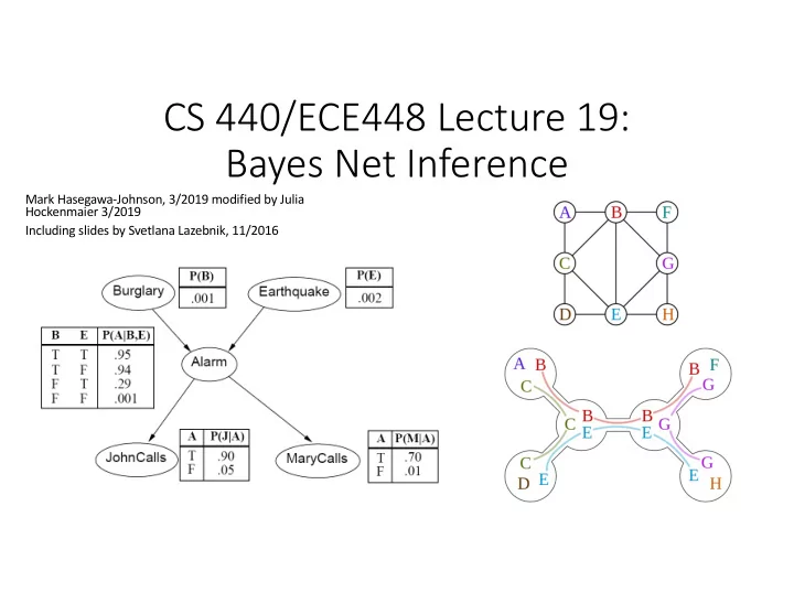
CS 440/ECE448 Lecture 19: Bayes Net Inference Mark - - PowerPoint PPT Presentation

CS 440/ECE448 Lecture 19: Bayes Net Inference

Mark Hasegawa-Johnson, 3/2019 modified by Julia Hockenmaier 3/2019 Including slides by Svetlana Lazebnik, 11/2016

CS440/ECE448 Lecture 19: Bayesian Networks and Bayes Net Inference

Slides by Svetlana Lazebnik, 10/2016 Modified by Mark Hasegawa-Johnson, 3/2019 and Julia Hockenmaier 3/2019

Today’s lecture

• Bayesian Networks (Bayes Nets)
• A graphical representation
• f probabilistic models
• Capture conditional (in)dependencies between random variables
• Inference and Learning in Bayes Nets
• Inference = Reasoning
• Learning = Parameter estimation

3 CS440/ECE448: Intro AI

Review: Bayesian inference

A general scenario:

Query variables: X Evidence (observed) variables and their values: E = e

Inference problem: answer questions about the query variables given the evidence variables This can be done using the posterior distribution P(X | E = e) Example of a useful question: Which X is true? More formally: what value of X has the least probability of being wrong? Answer: MPE = MAP (argmin P(error) = argmax P(X=x|E=e))

Today: What if P(X,E) is complicated?

• Very, very common problem: P(X,E) is complicated because both X

and E depend on some hidden variable Y

• SOLUTION:
• Represent the dependencies as a graph
• When your algorithm performs inference, make sure it does so in the order of

the graph

• FORMALISM: Bayesian Network

Bayesian Inference with Hidden Variables

• A general scenario:
• Query variables: X
• Evidence (observed) variables and their values: E = e
• Hidden (unobserved) variables: Y
• Inference problem: answer questions about the query

variables given the evidence variables

• This can be done using the posterior distribution P(X | E = e)
• In turn, the posterior needs to be derived from the full joint P(X, E, Y)
• Bayesian networks are a tool for representing joint

probability distributions efficiently

å

µ = =

y

y e X e e X e E X ) , , ( ) ( ) , ( ) | ( P P P P

Bayesian Networks

Bayesian networks

• More commonly called graphical models
• A way to depict conditional independence

relationships between random variables

• A compact specification of full joint distributions

Independence

• Random variables X and Y are independent (X⊥Y)

if P(X,Y) = P(X) × P(Y)

NB.: Since X and Y are R.V.s (not individual events), P(X,Y) = P(X)×P(Y) is an abbreviation for: ∀x∀y P(X=x,Y=y) =P(X=x)×P(Y=y)

• X and Y are conditionally independent given Z (X⊥Y | Z)

if P(X,Y | Z) = P(X | Z ) × P(Y | Z)

The value of X depends on the value of Z, and the value of Y depends on the value of Z, so X and Y are not independent.

9 CS440/ECE448: Intro AI

Bayesian networks

• Insight: (Conditional) independence assumptions are essential for

probabilistic modeling

• Bayes Net: a directed graph which represents the joint distribution of

a number of random variables in a directed graph

• Nodes = random variables
• Directed edges = dependencies

10 CS440/ECE448: Intro AI

Bayesian networks

• Nodes: random variables
• Edges: dependencies
• An edge from one variable (parent) to

another (child) indicates direct influence (conditional probabilities)

• Edges must form a directed, acyclic graph
• Each node is conditioned on its parents:

P(X | Parents(X)) These conditional distributions are the parameters of the network

• Each node is conditionally independent
• f its non-descendants given its parent

We have four random variables Weather is independent of cavity, toothache and catch Toothache and catch both depend on cavity.

Conditional independence and the joint distribution

• Key property: each node is conditionally independent of

its non-descendants given its parents

• Suppose the nodes X1, …, Xn are sorted in topological order
• f the graph (i.e. if Xi is a parent of Xj, i < j)
• To get the joint distribution P(X1, …, Xn),

use chain rule (step 1 below) and then take advantage of independencies (step 2)

( )

Õ

=

• =

n i i i n

X X X P X X P

1 1 1 1

, , | ) , , ( ! !

( )

Õ

=

=

n i i i

X Parents X P

1

) ( |

The joint probability distribution

P(j, m, a, ¬b,¬e) = P(¬b) P(¬e) P(a|¬b,¬e) P(j|a) P(m|a)

( )

Õ

=

=

n i i i n

X Parents X P X X P

1 1

) ( | ) , , ( !

Example: N independent coin flips

• Complete independence: no interactions:

P(X1) P(X2) P(X3)

X1 X2 Xn

…

Conditional probability distributions

• To specify the full joint distribution, we need to specify a

conditional distribution for each node given its parents:

P (X| Parents(X))

Z1 Z2 Zn

X

…

P (X| Z1, …, Zn)

Naïve Bayes document model

• Random variables:
• X: document class
• W1, …, Wn: words in the document
• Dependencies: P(X) P(W1 | X) … P(Wn | X)

W1 W2 Wn

…

X

Example: Los Angeles Burglar Alarm

• I have a burglar alarm that is sometimes set off by minor earthquakes. My two

neighbors, John and Mary, promised to call me at work if they hear the alarm

• Example inference task: suppose Mary calls and John doesn’t call. What is the probability of a

burglary?

• What are the random variables?
• Burglary, Earthquake, Alarm, JohnCalls, MaryCalls
• What are the direct influence relationships?
• A burglar can set the alarm off
• An earthquake can set the alarm off
• The alarm can cause Mary to call
• The alarm can cause John to call

Example: Burglar Alarm

𝑄(𝐶) 𝑄(𝐹) 𝑄(𝐵|𝐶, 𝐹) 𝑄(𝑁|𝐵) 𝑄(𝐾|𝐵)

• A “model” is a complete

specification of the dependencies.

• The conditional

probability tables are the model parameters.

Example: Burglar Alarm

Outline

• Review: Bayesian inference
• Bayesian network: graph semantics
• The Los Angeles burglar alarm example
• Conditional independence ≠ Independence
• Constructing a Bayesian network: Structure learning
• Constructing a Bayesian network: Hire an expert

Independence

• By saying that 𝑌/ and 𝑌

0 are independent, we mean that

P(𝑌

0, 𝑌/) = P(𝑌/)P(𝑌 0)

• 𝑌/ and 𝑌

0 are independent if and only if they have no common

ancestors

• Example: independent coin flips
• Another example: Weather is independent of all other variables in this

model.

X1 X2 Xn

…

Conditional independence

• By saying that 𝑋

/ and 𝑋 0 are conditionally independent given 𝑌, we

mean that P 𝑋

/, 𝑋 0 𝑌 = P(𝑋 /|𝑌)P(𝑋 0|𝑌)

• 𝑋

/ and 𝑋 0 are conditionally independent given 𝑌 if and only if they

have no common ancestors other than the ancestors of 𝑌.

• Example: naïve Bayes model:

W1 W2 Wn

…

X

Common cause: Conditionally Independent Common effect: Independent

Are X and Z independent? No 𝑄 𝑎, 𝑌 = 5

6

𝑄 𝑎 𝑍 𝑄 𝑌 𝑍 𝑄(𝑍) 𝑄 𝑎 𝑄 𝑌 = 5

6

𝑄 𝑎 𝑍 𝑄(𝑍) 5

6

𝑄 𝑌 𝑍 𝑄(𝑍) Are they conditionally independent given Y? Yes 𝑄 𝑎, 𝑌 𝑍 = 𝑄(𝑎|𝑍)𝑄(𝑌|𝑍)

Are X and Z independent? Yes 𝑄(𝑌, 𝑎) = 𝑄(𝑌)𝑄(𝑎) Are they conditionally independent given Y? No 𝑄 𝑎, 𝑌 𝑍 = 𝑄 𝑍 𝑌, 𝑎 𝑄 𝑌 𝑄(𝑎) 𝑄(𝑍) ≠ 𝑄 𝑎|𝑍 𝑄 𝑌|𝑍

Conditional independence ≠ Independence

Common cause: Conditionally Independent Common effect: Independent

Are X and Z independent? No Knowing X tells you about Y, which tells you about Z. Are they conditionally independent given Y? Yes If you already know Y, then X gives you no useful information about Z. Are X and Z independent? Yes Knowing X tells you nothing about Z. Are they conditionally independent given Y? No If Y is true, then either X or Z must be true. Knowing that X is false means Z must be true. We say that X “explains away” Z.

Conditional independence ≠ Independence

Conditional independence ≠ Independence

Being conditionally independent given X does NOT mean that 𝑋

/ and 𝑋 0 are

• independent. Quite the opposite. For example:
• The document topic, X, can be either “sports” or “pets”, equally probable.
• W1=1 if the document contains the word “food,” otherwise W1=0.
• W2=1 if the document contains the word “dog,” otherwise W2=0.
• Suppose you don’t know X, but you know that W2=1 (the document has the

word “dog”). Does that change your estimate of p(W1=1)?

W1 W2 Wn

…

X

Conditional independence

Another example: causal chain

• X and Z are conditionally independent given Y, because they have

no common ancestors other than the ancestors of Y.

• Being conditionally independent given Y does NOT mean that X

and Z are independent. Quite the opposite. For example, suppose P(𝑌) = 0.5, P 𝑍 𝑌 = 0.8, P 𝑍 ¬𝑌 = 0.1, P 𝑎 𝑍 = 0.7, and P 𝑎 ¬𝑍 = 0.4. Then we can calculate that P 𝑎 𝑌 = 0.64, but P(𝑎) = 0.535

Outline

• Review: Bayesian inference
• Bayesian network: graph semantics
• The Los Angeles burglar alarm example
• Conditional independence ≠ Independence
• Constructing a Bayesian network: Structure learning
• Constructing a Bayesian network: Hire an expert

Constructing a Bayes Network: Two Methods

• 1. “Structure Learning” a.k.a. “Analysis of Causality:”

1. Suppose you know the variables, but you don’t know which variables depend on which others. You can learn this from data. 2. This is an exciting new area of research in statistics, where it goes by the name of “analysis of causality.” 3. … but it’s almost always harder than method #2. You should know how to do this in very simple examples (like the Los Angeles burglar alarm), but you don’t need to know how to do this in the general case.

• 2. “Hire an Expert:”

1. Find somebody who knows how to solve the problem. 2. Get her to tell you what are the important variables, and which variables depend

• n which others.

3. THIS IS ALMOST ALWAYS THE BEST WAY.

Constructing Bayesian networks: Structure Learning

• 1. Choose an ordering of variables X1, … , Xn
• 2. For i = 1 to n
• add Xi to the network
• Check your training data. If there is any variable X1, … ,Xi-1 that CHANGES

the probability of Xi=1, then add that variable to the set Parents(Xi) such that P(Xi | Parents(Xi)) = P(Xi | X1, ... Xi-1) 3. Repeat the above steps for every possible ordering (complexity: n!). 4. Choose the graph that has the smallest number of edges.

• Suppose we choose the ordering M, J, A, B, E

Example

• Suppose we choose the ordering M, J, A, B, E

Example

• Suppose we choose the ordering M, J, A, B, E

Example

• Suppose we choose the ordering M, J, A, B, E

Example

• Suppose we choose the ordering M, J, A, B, E

Example

• Suppose we choose the ordering M, J, A, B, E

Example

• Suppose we choose the ordering M, J, A, B, E

Example

• Suppose we choose the ordering M, J, A, B, E

Example

Example contd.

• Deciding conditional independence is hard in noncausal directions
• The causal direction seems much more natural
• Network is less compact: 1 + 2 + 4 + 2 + 4 = 13 numbers needed (vs.

1+1+4+2+2=10 for the causal ordering)

versus

Why store it in causal order? A: Saves memory

• Suppose we have a Boolean variable Xi with k Boolean parents. How many rows

does its conditional probability table have?

• 2k rows for all the combinations of parent values
• Each row requires one number for P(Xi = true | parent values)
• If each variable has no more than k parents, how many numbers does the

complete network require?

• O(n · 2k) numbers – vs. O(2n) for the full joint distribution
• How many nodes for the burglary network?

1 + 1 + 4 + 2 + 2 = 10 numbers (vs. 25-1 = 31)

Outline

• Review: Bayesian inference
• Bayesian network: graph semantics
• The Los Angeles burglar alarm example
• Conditional independence ≠ Independence
• Constructing a Bayesian network: Structure learning
• Constructing a Bayesian network: Hire an expert

A more realistic Bayes Network: Car diagnosis

• Initial observation: car won’t start
• Orange: “broken, so fix it” nodes
• Green: testable evidence
• Gray: “hidden variables” to ensure sparse structure, reduce parameters

Car insurance

In research literature…

Causal Protein-Signaling Networks Derived from Multiparameter Single-Cell Data Karen Sachs, Omar Perez, Dana Pe'er, Douglas A. Lauffenburger, and Garry P. Nolan (22 April 2005) Science 308 (5721), 523.

In research literature…

Describing Visual Scenes Using Transformed Objects and Parts

• E. Sudderth, A. Torralba, W. T. Freeman, and A. Willsky.

International Journal of Computer Vision, No. 1-3, May 2008, pp. 291-330.

In research literature…

Audiovisual Speech Recognition with Articulator Positions as Hidden Variables Mark Hasegawa-Johnson, Karen Livescu, Partha Lal and Kate Saenko International Congress on Phonetic Sciences 1719:299-302, 2007

In research literature…

Detecting interaction links in a collaborating group using manually annotated data

• S. Mathur, M.S. Poole, F. Pena-Mora, M. Hasegawa-Johnson, N. Contractor

Social Networks 10.1016/j.socnet.2012.04.002

In research literature…

Detecting interaction links in a collaborating group using manually annotated data

• S. Mathur, M.S. Poole, F. Pena-Mora, M. Hasegawa-Johnson, N. Contractor

Social Networks 10.1016/j.socnet.2012.04.002

• Link: 𝑀/0 = 1 if #i is

listening to #j.

• Indirect: 𝐽/0 = 1 if

#i and #j are both listening to the same person.

• Speaking: 𝑇/ = 1 if

the i’th person is speaking.

• Gaze: 𝐻/0 = 1 if #i

is looking at #j.

• Neighborhood:

𝑂/0 = 1 if they’re near one another

Summary

• Bayesian networks provide a natural representation for (causally

induced) conditional independence

• Topology + conditional probability tables
• Generally easy for domain experts to construct

CS 440/ECE448 Lecture 19: Bayes Net Inference

Mark Hasegawa-Johnson, 3/2019 modified by Julia Hockenmaier 3/2019 Including slides by Svetlana Lazebnik, 11/2016

Bayes Net Inference and Learning

Bayes Network Inference & Learning

Bayes net is a memory-efficient model of dependencies among a set

• f random variables.

Inference problem: answer questions about the query variables X given the evidence variables and their values E=e as well as some unobserved (hidden) variables Y.

• We want to know the posterior distribution P(X | E = e)
• The posterior can be derived from the full joint P(X, E, Y)
• How do we make this computationally efficient?

Learning problem: given some training examples, how do we estimate the parameters of the model?

• Parameters = p(variable|parents), for each variable in the net

Outline

• Inference Examples
• Inference Algorithms
• Trees: Sum-product algorithm
• Poly-trees: Junction tree algorithm
• Graphs: No polynomial-time algorithm
• Parameter Learning

Practice example 1

• Variables: Cloudy, Sprinkler, Rain, Wet Grass

Practice example 1

• Given that the grass is wet, what is the probability

that it has rained?

P(r | w) = P(r,w) P(w) = P(c,s,r,w)

C=c,S=s

∑

P(c,s,r,w)

C=c,S=s,R=r

∑

= P(c)P(s | c)P(r | c)P(w | r,s)

C=c,S=s

∑

P(c)P(s | c)P(r | c)P(w | r,s)

C=c,S=s,R=r

∑

Practice example 1

• Given that the grass is wet, what is the probability

that it has rained?

P(r | w) = P(r,w) P(w) = P(c,s,r,w)

C=c,S=s

∑

P(c,s,r,w)

C=c,S=s,R=r

∑

= P(c)P(s | c)P(r | c)P(w | r,s)

C=c,S=s

∑

P(c)P(s | c)P(r | c)P(w | r,s)

C=c,S=s,R=r

∑

Practice example 1

• Given that the grass is wet, what is the probability

that it has rained?

P(r | w) = P(r,w) P(w) = P(c,s,r,w)

C=c,S=s

∑

P(c,s,r,w)

C=c,S=s,R=r

∑

= P(c)P(s | c)P(r | c)P(w | r,s)

C=c,S=s

∑

P(c)P(s | c)P(r | c)P(w | r,s)

C=c,S=s,R=r

∑

Practice Example #2

• Suppose you have an observation, for example, “Jack called” (J=1)
• You want to know: was there a burglary?
• You need

𝑄 𝐶 = 1 𝐾 = 1 = 𝑄(𝐶, 𝐾 = 1) ∑H 𝑄(𝐶 = 𝑐, 𝐾 = 1)

• So you need to compute the table P(B,J) for all possible settings of

(B,J)

Bayes Net Inference: The Hard Way

• 1. P(B, E, A, J, M) = P(B) P(E) P(A|B,E) P(J|A) P(M|A)
• 2. P B, J = ∑Q ∑R ∑S P(B, E, A, J, M)

Exponential complexity (#P-hard, actually): N variables, each of which has K possible values ⇒ 𝑃{𝐿X} time complexity

Is there an easier way?

• Tree-structured Bayes nets: the sum-product algorithm
• Quadratic complexity, 𝑃{𝑂𝐿Z}
• Polytrees: the junction tree algorithm
• Pseudo-polynomial complexity, 𝑃{𝑂𝐿[}, for M<N
• Arbitrary Bayes nets: #P complete, 𝑷{𝑳𝑶}
• The SAT problem is a Bayes net!

• 1. Tree-Structured Bayes Nets
• Suppose these are all binary variables.
• We observe E=1
• We want to find P(H=1|E=1)
• Means that we need to find both

P(H=0,E=1) and P(H=1,E=1) because 𝑄 𝐼 = 1 𝐹 = 1 = 𝑄(𝐼 = 1, 𝐹 = 1) ∑` 𝑄(𝐼 = ℎ, 𝐹 = 1)

The Sum-Product Algorithm (Belief Propagation)

• Find the only undirected path from the

evidence variable to the query variable (E-D-B-F-G-I-H)

• Find the directed root of this path P(F)
• Find the joint probabilities of root and

evidence: P(F=0,E=1) and P(F=1,E=1)

• Find the joint probabilities of query and

evidence: P(H=0,E=1) and P(H=1,E=1)

• Find the conditional probability P(H=1|E=1)

The Sum-Product Algorithm

Starting with the root P(F), we find P(F,E) by alternating product steps and sum steps:

• 1. Product: P(B,D,F)=P(F)P(B|F)P(D|B)
• 2. Sum: 𝑄 𝐸, 𝐺 = ∑fgh

i

𝑄(𝐶, 𝐸, 𝐺)

• 3. Product: P(D,E,F)=P(D,F)P(E|D)
• 4. Sum: 𝑄 𝐹, 𝐺 = ∑jgh

i

𝑄(𝐸, 𝐹, 𝐺)

The Sum-Product Algorithm (Belief Propagation)

The Sum-Product Algorithm

Starting with the root P(E,F), we find P(E,H) by alternating product steps and sum steps:

• 1. Product: P(E,F,G)=P(E,F)P(G|F)
• 2. Sum: 𝑄 𝐹, 𝐻 = ∑lgh

i

𝑄(𝐹, 𝐺, 𝐻)

• 3. Product: P(E,G,I)=P(E,G)P(I|G)
• 4. Sum: 𝑄 𝐹, 𝐽 = ∑ngh

i

𝑄(𝐹, 𝐻, 𝐽)

• 5. Product: P(E,H,I)=P(E,I)P(I|G)
• 6. Sum: 𝑄 𝐹, 𝐼 = ∑pgh

i

𝑄(𝐹, 𝐼, 𝐽)

The Sum-Product Algorithm (Belief Propagation)

• Each product step generates a table

with 3 variables

• Each sum step reduces that to a table

with 2 variables

• If each variable has K values, and if there

are 𝑃{𝑂} variables on the path from evidence to query, then time complexity is 𝑃{𝑂𝐿Z}

Time Complexity of Belief Propagation

Time Complexity of Bayes Net Inference

• Tree-structured Bayes nets: the sum-product algorithm
• Quadratic complexity, 𝑃{𝑂𝐿Z}
• Polytrees: the junction tree algorithm
• Pseudo-polynomial complexity, 𝑃{𝑂𝐿[}, for M<N
• Arbitrary Bayes nets: #P complete, 𝑷{𝑳𝑶}
• The SAT problem is a Bayes net!

• 2. The Junction Tree Algorithm
• a. Moralize the graph (identify each variable’s Markov blanket)
• b. Triangulate the graph (eliminate undirected cycles)
• c. Create the junction tree (form cliques)
• d. Run the sum-product algorithm on the junction tree

2.a. Markov Blanket

• Suppose there is a Bayes net

with variables A,B,C,D,E,F,G,H

• The “Markov blanket” of

variable F is D,E,G if P(F|A,B,C,D,E,G,H) = P(F|D,E,G)

2.a. Markov Blanket

• Suppose there is a Bayes net

with variables A,B,C,D,E,F,G,H

• The “Markov blanket” of

variable F is D,E,G if P(F|A,B,C,D,E,G,H) = P(F|D,E,G)

A B C D E F G H

2.a. Markov Blanket

• The “Markov blanket” of variable F is

D,E,G if P(F|A,B,C,D,E,G,H) = P(F|D,E,G)

• How can we prove that?
• P(A,…,H) = P(A)P(B|A) …
• Which of those terms include F?

A B C D E F G H

2.a. Markov Blanket

• Which of those terms include F?
• Only these two:

P(F|D) and P(G|E,F)

A B C D E F G H

2.a. Markov Blanket

The Markov Blanket of variable F includes only its immediate family members:

• Its parent, D
• Its child, G
• The other parent of its child, E

Because P(F|A,B,C,D,E,G,H) = P(F|D,E,G)

A B C D E F G H

2.a. Moralization

“Moralization” =

• 1. If two variables have a child

together, force them to get married.

• 2. Get rid of the arrows (not

necessary any more). Result: Markov blanket = the set of variables to which a variable is connected.

A B C D E F G H

2.b. Triangulation

Triangulation = draw edges so that there is no unbroken cycle of length > 3. There are usually many different ways to do this. For example, here’s one:

A B C D E F G H

2.c. Form Cliques

Clique = a group of variables, all of whom are members of each other’s immediate family. Junction Tree = a tree in which

• Each node is a clique from the
• riginal graph,
• Each edge is an “intersection set,”

naming the variables that overlap between the two cliques.

A B C D E F G H AB BCD CDF CEF EFG GH

B CD CF EF G

2.d. Sum-Product

Suppose we need P(B,G):

• 1. Product: P(B,C,D,F)=P(B)P(C|B)P(D|B)P(F|D)
• 2. Sum: 𝑄 𝐶, 𝐷, 𝐺 = ∑j 𝑄(𝐶, 𝐷, 𝐸, 𝐺)
• 3. Product: P(B,C,E,F)=P(B,C,F)P(E|C)
• 4. Sum: 𝑄 𝐶, 𝐹, 𝐺 = ∑s 𝑄(𝐶, 𝐷, 𝐹, 𝐺)
• 5. Product: P(B,E,F,G) = P(B,E,F)P(G|E,F)
• 6. Sum: 𝑄 𝐶, 𝐻 = ∑t ∑l 𝑄(𝐶, 𝐹, 𝐺, 𝐻)

Complexity: 𝑃{𝑂𝐿[}, where N=# cliques, K = # values for each variable, M = 1 + # variables in the largest clique

B C D E F G

Junction Tree: Sample Test Question

Consider the burglar alarm example.

• a. Moralize this graph
• b. Is it already triangulated? If

not, triangulate it.

• c. Draw the junction tree

Solution B E A J M

Solution

• a. Moralize this graph

B E A J M

Solution

• b. Is it already triangulated?

Answer: yes. There is no unbroken cycle of length > 3.

B E A J M

Solution

• c. Draw the junction tree

ABE AJ AM

A A

Time Complexity of Bayes Net Inference

• Tree-structured Bayes nets: the sum-product algorithm
• Quadratic complexity, 𝑃{𝑂𝐿Z}
• Polytrees: the junction tree algorithm
• Pseudo-polynomial complexity, 𝑃{𝑂𝐿[}, for M<N
• Arbitrary Bayes nets: #P complete, 𝑷{𝑳𝑶}
• The SAT problem is a Bayes net!

Bayesian network inference

• In full generality, NP-hard
• More precisely, #P-hard: equivalent to counting satisfying assignments
• We can reduce satisfiability to Bayesian network inference
• Decision problem: is P(Y) > 0?

Y = (U1 ∨U2 ∨U3)∧(¬U1 ∨¬U2 ∨U3)∧(U2 ∨¬U3 ∨U4)

Bayesian network inference

• In full generality, NP-hard
• More precisely, #P-hard: equivalent to counting satisfying assignments
• We can reduce satisfiability to Bayesian network inference
• Decision problem: is P(Y) > 0?
• G. Cooper, 1990

Y = (U1 ∨U2 ∨U3)∧(¬U1 ∨¬U2 ∨U3)∧(U2 ∨¬U3 ∨U4)

C1 C2 C3

Bayesian network inference

P(U1,U2,U3,U4,C1,C2,C3, D1, D2,Y) = P(U1)P(U2)P(U3)P(U4) P(C1 |U1,U2,U3)P(C2 |U1,U2,U3)P(C3 |U2,U3,U4) P(D1 |C1)P(D2 | D1,C2)P(Y | D2,C3)

Bayesian network inference

Why can’t we use the junction tree algorithm to efficiently compute Pr(Y)?

Bayesian network inference

Why can’t we use the junction tree algorithm to efficiently compute Pr(Y)? Answer: after we moralize and triangulate, the size of the largest clique (u2u3c1c2c3) is 𝑁 ≈ 𝑂, same order

• f magnitude as the original problem

Time Complexity of Bayes Net Inference

• Tree-structured Bayes nets: the sum-product algorithm
• Quadratic complexity, 𝑃{𝑂𝐿Z}
• Polytrees: the junction tree algorithm
• Pseudo-polynomial complexity, 𝑃{𝑂𝐿[}, for M<N
• Arbitrary Bayes nets: #P complete, 𝑃{𝐿X}
• The SAT problem is a Bayes net!

Parameter learning

• Inference problem: given values of evidence variables

E = e, answer questions about query variables X using the posterior P(X | E = e)

• Learning problem: estimate the parameters of the

probabilistic model P(X | E) given a training sample {(x1,e1), …, (xn,en)}

Parameter learning: complete data

• Suppose we know the network structure (but not the

parameters), and have a training set of complete

• bservations

Sample

C S R W 1 T F T T 2 F T F T 3 T F F F 4 T T T T 5 F T F T 6 T F T F … … … …. …

? ? ? ? ? ? ? ? ?

Training set

Parameter learning

• Suppose we know the network structure (but not the

parameters), and have a training set of complete

• bservations
• Example:

𝑄 𝑇 = 𝑈 𝐷 = 𝑈 = #samples with 𝑇 = 𝑈, 𝐷 = 𝑈 # samples with 𝐷 = 𝑈 = 1 4

Sample

C S R W 1 T F T T 2 F T F T 3 T F F F 4 T T T T 5 F T F T 6 T F T F … … … …. …

Training set

Parameter learning

• Suppose we know the network structure (but not the

parameters), and have a training set of complete

• bservations
• P(X | Parents(X)) is given by the observed frequencies of

the different values of X for each combination of parent values

Parameter learning: missing data

• Suppose we know the network structure (but not the

parameters), and have a training set, but the training set is missing some observations.

? ? ? ? ? ? ? ? ?

Training set

Sample

C S R W 1 ? F T T 2 ? T F T 3 ? F F F 4 ? T T T 5 ? T F T 6 ? F T F … … … …. …

Missing data: the EM algorithm

• The EM algorithm starts (“Expectation Maximization”)

starts with an initial guess for each parameter value.

• We try to improve the initial guess, using the algorithm on the

next two slides:

• E-step
• M-step

0.5? 0.5? 0.5? 0.5? 0.5? 0.5? 0.5? 0.5? 0.5?

Training set

Sample

C S R W 1 ? F T T 2 ? T F T 3 ? F F F 4 ? T T T 5 ? T F T 6 ? F T F … … … …. …

Missing data: the EM algorithm

• E-Step (Expectation): Given the model parameters, replace each of the missing

numbers with a probability (a number between 0 and 1) using 𝑄 𝐷 = 1 𝑇, 𝑆, 𝑋 = 𝑄(𝐷 = 1, 𝑇, 𝑆, 𝑋) 𝑄 𝐷 = 1, 𝑇, 𝑆, 𝑋 + 𝑄(𝐷 = 0, 𝑇, 𝑆, 𝑋)

0.5? 0.5? 0.5? 0.5? 0.5? 0.5? 0.5? 0.5? 0.5?

Training set

Sample

C S R W 1 0.5? F T T 2 0.5? T F T 3 0.5? F F F 4 0.5? T T T 5 0.5? T F T 6 0.5? F T F … … … …. …

Missing data: the EM algorithm

• M-Step (Maximization): Given the missing data estimates, replace each of the

missing model parameters using 𝑄 Variable = T Parents = value = 𝐹[# times Variable = 𝑈, Parents = value] 𝐹[#times Parents = value]

0.5 0.5 0.5 0.5 0.5 1.0 1.0 0.5 0.0

Training set

Sample

C S R W 1 0.5? F T T 2 0.5? T F T 3 0.5? F F F 4 0.5? T T T 5 0.5? T F T 6 0.5? F T F … … … …. …

Missing data: the EM algorithm

• Iterate back and forth between E-step and M-step until the model converges.

0.5 0.5 0.5 0.5 0.5 1.0 1.0 0.5 0.0

Training set

Sample

C S R W 1 0.5? F T T 2 0.5? T F T 3 0.5? F F F 4 0.5? T T T 5 0.5? T F T 6 0.5? F T F … … … …. …

Summary: Bayesian networks

• Structure
• Parameters
• Inference
• Learning