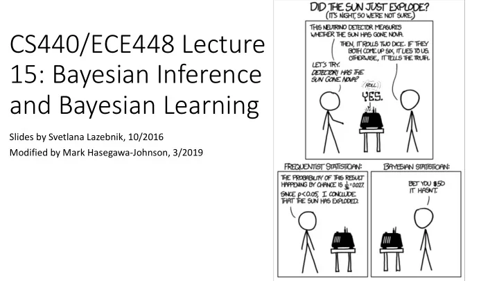
CS440/ECE448 Lecture 15: Bayesian Inference and Bayesian Learning - - PowerPoint PPT Presentation

CS440/ECE448 Lecture 15: Bayesian Inference and Bayesian Learning

Slides by Svetlana Lazebnik, 10/2016 Modified by Mark Hasegawa-Johnson, 3/2019

Bayesian Inference and Bayesian Learning

• Bayes Rule
• Bayesian Inference
• Misdiagnosis
• The Bayesian “Decision”
• The “Naïve Bayesian” Assumption
• Bag of Words (BoW)
• Bayesian Learning
• Maximum Likelihood estimation of parameters
• Maximum A Posteriori estimation of parameters
• Laplace Smoothing

Bayes’ Rule

• The product rule gives us two ways to factor

a joint probability: ! ", $ = ! $ " ! " = ! " $ ! $

• Therefore,

! " $ = ! $ " !(") !($)

• Why is this useful?
• “A” is something we care about, but P(A|B) is really really hard to measure

(example: the sun exploded)

• “B” is something less interesting, but P(B|A) is easy to measure (example: the

amount of light falling on a solar cell)

• Bayes’ rule tells us how to compute the probability we want (P(A|B)) from

probabilities that are much, much easier to measure (P(B|A)).

• Rev. Thomas Bayes

(1702-1761)

Bayes Rule example

Eliot & Karson are getting married tomorrow, at an outdoor ceremony in the desert.

• In recent years, it has rained only 5 days each year (5/365 = 0.014).

! " = 0.014 and ! ¬" = 0.956

• Unfortunately, the weatherman has predicted rain for tomorrow.

When it actually rains, the weatherman (correctly) forecasts rain 90% of the time. ! , " = 0.9

• When it doesn't rain, he (incorrectly) forecasts rain 10% of the time.

! , ¬" = 0.1

• What is the probability that it will rain on Eliot’s wedding if rain is forecast?

! " , = ! , " !(") !(,) = ! ,, " !(") ! ,, " + !(,, ¬") = ! , " !(") ! ,|" !(") + ! , ¬" !(¬") = (0.9)(0.014) 0.9 0.014 + (0.1)(0.956) = 0.116

The More Useful Version

• f Bayes’ Rule

! " # = ! # " !(") !(#)

• Remember, ' (|* is easy to measure

(the probability that light hits our solar cell, if the sun still exists and it’s daytime).

• Let’s assume we also know ' * (the probability the sun still exists).
• But suppose we don’t really know ' ( (what is the probability light hits our solar

cell, if we don’t really know whether the sun still exists or not?)

• However, we can compute ' ( = ' ( * ' * + ' ( ¬* ' ¬*

! " # = ! # " !(") ! # " ! " + ! # ¬" ! ¬"

• Rev. Thomas Bayes

(1702-1761)

This version is what you memorize. This version is what you actually use.

Bayesian Inference and Bayesian Learning

• Bayes Rule
• Bayesian Inference
• Misdiagnosis
• The Bayesian “Decision”
• The “Naïve Bayesian” Assumption
• Bag of Words (BoW)
• Bayesian Learning
• Maximum Likelihood estimation of parameters
• Maximum A Posteriori estimation of parameters
• Laplace Smoothing

The Misdiagnosis Problem

• 1% of women at age forty who participate in routine screening have breast cancer.
• 80% of women with breast cancer will get positive mammographies.
• 9.6% of women without breast cancer will also get positive mammographies.
• A woman in this age group had a positive mammography in a routine screening.

What is the probability that she actually has breast cancer? P(cancer | positive) = P(positive | cancer)P(cancer) P(positive) 0776 . 095 . 008 . 008 . 99 . 096 . 01 . 8 . 01 . 8 . = + = ´ + ´ ´ = = P(positive | cancer)P(cancer) P(positive | cancer)P(cancer)+ P(positive | ¬cancer)P(¬Cancer)

CHECK YOUR SYMPTOMS FIND A DOCTOR FIND LOWEST DRUG PRICES

HEALTH A-Z DRUGS & SUPPLEMENTS LIVING HEALTHY FAMILY & PREGNANCY NEWS & EXPERTS

To Get Health

ADVERTISEMENT

HEALTH INSURANCE AND MEDICARE HOME

News Reference Quizzes Videos Message Boards Find a Doctor

RELATED TO HEALTH INSURANCE

Health Insurance and Medicare ! Reference !

Second Opinions

If your doctor tells you that you have a health problem or suggests a treatment for an illness or injury, you might want a second opinion. This is especially true when you're considering surgery or major procedures. Asking another doctor to review your case can be useful for many reasons:

" # $

% & '

TODAY ON WEBMD

Clinical Trials

What qualifies you for one?

Working During Cancer Treatment

Know your benefits.

Going to the Dentist?

How to save money.

Enrolling in Medicare

How to get started.

SEARCH

(

SIGN IN

SUBSCRIBE

Considering Treatment for Illness, Injury? Get a Second Opinion https://www.webmd.com/health-insurance/second-opinions#1

The Bayesian Decision

The agent is given some evidence, ! and has to make a decision about the value of an unobserved variable ". " is called the “query variable” or the “class variable” or the “category.”

• Partially observable, stochastic, episodic environment
• Example: # ∈ {spam, not spam}, % = email message.
• Example: # ∈ {zebra, giraffe, hippo}, % = image features

The Bayesian Decision: Loss Function

• The query variable, Y, is a random variable.
• Assume its pmf, P(Y=y) is known.
• Furthermore, the true value of Y has already been determined
• -- we just don’t know what it is!
• The agent must act by saying “I believe that Y=a”.
• The agent has a post-hoc loss function !(#, %)
• !(#, %) is the incurred loss if the true value is Y=y, but the agent says “a”
• The a priori loss function !(', %) is a binary random variable
• ((!(', %) = 0) = ((' = %)
• ((!(', %) = 1) = ((' ≠ %)

Loss Function Example

• Suppose Y=outcome of a coin toss.
• The agent will choose the action “a”

(which is either a=heads, or a=tails)

• The loss function L(y,a) is
• Suppose we know that the coin is biased, so that

P(Y=heads)=0.6. Therefore the agent chooses a=heads. The loss function L(Y,a) is now a random variable:

L(y,a) y=heads y=tails a=heads 1 a=tails 1 c=0 c=1 P(L(Y,a)=c) 0.6 0.4

The Bayesian Decision

• The observation, E, is another random variable.
• Suppose the joint probability !(# = %, ' = () is known.
• The agent is allowed to observe the true value of E=e

before it guesses the value of Y.

• Suppose that the observed value of E is E=e.

Suppose the agent guesses that Y=a.

• Then its loss, L(Y,a), is a conditional random variable:

!(*(#, +) = 0|' = () = !(# = +|' = () ! * #, + = 1 ' = ( = ! # ≠ + ' = ( = ∑123 !(# = %|' = ()

• Suppose the agent chooses any particular action “a”.

Then its expected loss is:

! "($, &) ! = ) = *

+

" ,, & - $ = , ! = ) = *

+./

• $ = , ! = )
• Which action “a” should the agent choose

in order to minimize its expected loss?

• The one that has the greatest posterior probability.

The best value of “a” to choose is the one given by: & = arg max

/

• ($ = &|! = ))
• This is called the Maximum a Posteriori (MAP) decision

The Bayesian Decision

The action, “a”, should be the value of C that has the highest posterior probability given the observation X=x:

!

∗= argmax! ) * = ! + = , = argmax!

) + = , * = ! )(* = !) )(+ = ,) = argmax! ) + = , * = ! )(* = !)

MAP decision

Maximum Likelihood (ML) decision: !

∗ /0 = argmax a)(+ = ,|* = !)

Maximum A Posterior (MAP) decision: a* MAP = argmax! ) * = ! + = , = argmax!) + = , * = ! )(* = !)

likelihood prior posterior

The Bayesian Terms

• !(# = %) is called the “prior” (a priori, in Latin) because it represents

your belief about the query variable before you see any observation.

• ! # = % ' = ( is called the “posterior” (a posteriori, in Latin),

because it represents your belief about the query variable after you see the observation.

• ! ' = ( # = % is called the “likelihood” because it tells you how

much the observation, E=e, is like the observations you expect if Y=y.

• !(' = () is called the “evidence distribution” because E is the

evidence variable, and !(' = () is its marginal distribution. ! % ( = ! ( % !(%) !(()

Bayesian Inference and Bayesian Learning

• Bayes Rule
• Bayesian Inference
• Misdiagnosis
• The Bayesian “Decision”
• The “Naïve Bayesian” Assumption
• Bag of Words (BoW)
• Bayesian Learning
• Maximum Likelihood estimation of parameters
• Maximum A Posteriori estimation of parameters
• Laplace Smoothing

Naïve Bayes model

• Suppose we have many different types of observations

(symptoms, features) X1, …, Xn that we want to use to obtain evidence about an underlying hypothesis C

• MAP decision:

! " = $ %& = '&, … , %* = '* ∝ ! " = $ !(%& = '&, … , %* = '*|" = $)

• If each feature %/ can take on k values, how many entries are in

the pmf table !(%& = '&, … , %* = '*|" = $)?

Naïve Bayes model

• If each feature !" can take on k values,

how many entries are in the pmf table #(%&, … , %)|+)?

• Without any independence assumptions: -(-) − 1)

(- values of Y = +, -(-) − 1) possible combinations of %&, … , %))

• Naïve Bayes makes the simplifying assumption that the different features

are conditionally independent given the hypothesis: # %&, … , %) + ≈ # %& + # %3 + … # %) +

• If each observation and the hypothesis can take on k values,

how many entries do we need to store to compute # %&, … , %) + ?

• Each # %4 + requires (- − 1)×-

(- values of Y = +, - − 1 of !4 = %4)

• There are 6 of them, for a total space requirement: 6× - − 1 ×-

Naïve Bayes model

Suppose we have many different types of observations (symptoms, features) E1, …, En that we want to use to obtain evidence about an underlying hypothesis Y MAP decision: ! = argmax ( ) = ! *+ = ,+, … , */ = ,/ = argmax ( ) = ! ( *+ = ,+, … , */ = ,/ ) = ! ≈ argmax ( ) = ! ( 1+ ! ( 12 ! … ( 1/ !

Case study: Text document classification

• MAP decision: assign a document to the class with the highest posterior

P(class | document)

• Example: spam classification
• Classify a message as spam if P(spam | message) > P(¬spam | message)

Case study: Text document classification

• MAP decision: assign a document to the class with the highest

posterior P(class | document)

• We have P(class | document) µ P(document | class)P(class)
• To enable classification, we need to be able to estimate the likelihoods

P(document | class) for all classes and priors P(class)

Naïve Bayes Representation

• Goal: estimate likelihoods P(document | class)

and priors P(class)

• Likelihood: bag of words representation
• The document is a sequence of words (w1, …, wn)
• The order of the words in the document is not important
• Each word is conditionally independent of the others given document

class

Naïve Bayes Representation

• Goal: estimate likelihoods P(document | class)

and priors P(class)

• Likelihood: bag of words representation
• The document is a sequence of words (!" = w1, …, !$ = wn)
• The order of the words in the document is not important
• Each word is conditionally independent of the others given document

class

• Thus, the problem is reduced to estimating marginal likelihoods of

individual words p(wi | class)

P(document | class) = P(w1, ... ,wn | class) = P(wi | class)

i=1 n

∏

Parameter estimation

• Model parameters: feature likelihoods p(word | class) and priors

p(class)

• How do we obtain the values of these parameters?

spam: 0.33 ¬spam: 0.67 P(word | ¬spam) P(word | spam) prior

Bag of words illustration

US Presidential Speeches Tag Cloud http://chir.ag/projects/preztags/

Bag of words illustration

US Presidential Speeches Tag Cloud http://chir.ag/projects/preztags/

Bag of words illustration

US Presidential Speeches Tag Cloud http://chir.ag/projects/preztags/

Bayesian Inference and Bayesian Learning

• Bayes Rule
• Bayesian Inference
• Misdiagnosis
• The Bayesian “Decision”
• The “Naïve Bayesian” Assumption
• Bag of Words (BoW)
• Bayesian Learning
• Maximum Likelihood estimation of parameters
• Laplace Smoothing

• Model parameters: feature likelihoods P(word | class) and priors P(class)
• How do we obtain the values of these parameters?
• Need training set of labeled samples from both classes
• This is the maximum likelihood (ML) estimate, or estimate that

maximizes the likelihood of the training data:

Bayesian Learning

P(word | class) = # of occurrences of this word in docs from this class total # of words in docs from this class

ÕÕ

= = D d n i i d i d

d

class w P

1 1 , ,

) | (

d: index of training document, i: index of a word

Bayesian Learning

• The “bag of words model” has the following parameters:
• !"# ≡ %(' = )|+ = ,)
• ." ≡ %(+ = ,)
• The training data are a set of documents, / = [12, … , 15],

each with its associated class label, 7 = [+2, … , +5].

• The likelihood of the training data is the probability of its observations

given its labels. If we assume that each document is independent of the others (“episodic”), then we get: %(/, 7) = 8

9:2 5

% 19 +9 %(+9)

Bayesian Learning

• The “bag of words model” has the following parameters:
• !"# ≡ %(' = )|+ = ,)
• ." ≡ %(+ = ,)
• Each document is a sequence of words, /0 = ['

20, … , ' 50].

• If we assume that each word is conditionally independent given the class

(the naïve Bayes a.k.a. bag-of-words assumption), then we get: %(7, 8) = 9

0:2 ;

%(+0 = ,0) 9

<:2 5

%('

<0 = ) <0|+0 = ,0) = 9 0:2 ;

."= 9

<:2 5

!"=#>=

Bayesian Learning

The data likelihood !(#, %) is maximized if we choose:

'() = # occurrences of word 6 in documents of type < total number of words in all documents of type < @( = # documents of type < total number of documents

What is the probability that the sun will fail to rise tomorrow?

• # times we have observed the sun to rise = 100,000,000
• # times we have observed the sun not to rise = 0
• Estimated probability the sun will not rise =

! !"#!!,!!!,!!! = 0

Oops….

Laplace Smoothing

• The basic idea: add 1 “unobserved observation” to every possible

event

• # times the sun has risen or might have ever risen = 100,000,000+1 =

100,000,001

• # times the sun has failed to rise or might have ever failed to rise =

0+1 = 1

• Estimated probability the sun will not rise =

! !"!##,###,##! =

0.0000000099999998

Parameter estimation

• ML (Maximum Likelihood) parameter estimate:
• Laplacian Smoothing estimate
• How can you estimate the probability of a word you never saw in the training

set? (Hint: what happens if you give it probability 0, then it actually occurs in a test document?)

• Laplacian smoothing: pretend you have seen every vocabulary word one

more time than you actually did P(word | class) = # of occurrences of this word in docs from this class + 1 total # of words in docs from this class + V (V: total number of unique words) P(word | class) = # of occurrences of this word in docs from this class total # of words in docs from this class

Summary: Naïve Bayes for Document Classification

• Naïve Bayes model: assign the document to the class

with the highest posterior

• Model parameters:

P(class | document)∝ P(class) P(wi | class)

i=1 n

∏

P(class1) … P(classK) P(w1 | class1) P(w2 | class1) … P(wn | class1) Likelihood

• f class 1

prior P(w1 | classK) P(w2 | classK) … P(wn | classK) Likelihood

• f class K

…

Prediction

Bayesian Learning and Bayesian Inference irl:

Training Labels Training Samples Training

Learning

Features Features

Inference

Test Sample Learned model Learned model

Review: Bayesian decision making

• Suppose the agent has to make decisions about the

value of an unobserved query variable Y based on the values of an observed evidence variable E

• Inference problem: given some observation E = e,

what is P(Y | E=e)?

• Learning problem: estimate the parameters of the

probabilistic model P(y | e) given a training sample {(e1,y1), …, (en,yn)}