
SLIDE 1
CS440/ECE448 Lecture 15: Bayesian Networks
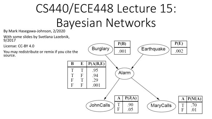
By Mark Hasegawa-Johnson, 2/2020 With some slides by Svetlana Lazebnik, 9/2017 License: CC-BY 4.0 You may redistribute or remix if you cite the source.
CS440/ECE448 Lecture 15: Bayesian Networks By Mark - - PowerPoint PPT Presentation
CS440/ECE448 Lecture 15: Bayesian Networks By Mark Hasegawa-Johnson, 2/2020 With some slides by Svetlana Lazebnik, 9/2017 License: CC-BY 4.0 You may redistribute or remix if you cite the source. Review: Bayesian inference A general
By Mark Hasegawa-Johnson, 2/2020 With some slides by Svetlana Lazebnik, 9/2017 License: CC-BY 4.0 You may redistribute or remix if you cite the source.
variables given the evidence variables
being wrong?
P(X=x|E=e))
and E depend on some hidden variable Y
the graph
variables given the evidence variables
probability distributions efficiently
µ = =
y
y e X e e X e E X ) , , ( ) ( ) , ( ) | ( P P P P
relationships between random variables
direct influence
X1 X2 Xn
W1 W2 Wn
X
neighbors, John and Mary, promised to call me at work if they hear the alarm
burglary?
non-descendants given its parents
use chain rule:
( )
=
n i i i n
X X X P X X P
1 1 1 1
, , | ) , , ( ! !
( )
=
=
n i i i
X Parents X P
1
) ( |
conditional distribution for each node given its parents:
P (X | Parents(X))
Z1 Z2 Zn
X
P (X | Z1, …, Zn)
specification of the dependencies.
probability tables are the model parameters.
Should you call the police?
called a MAP (maximum a posteriori) decision. You decide that you have a burglar in your house if and only if
𝑄 𝐶𝑣𝑠𝑚𝑏𝑠𝑧 𝑁𝑏𝑠𝑧 > 𝑄(¬𝐶𝑣𝑠𝑚𝑏𝑠𝑧|𝑁𝑏𝑠𝑧)
We have to figure out what it is.
¬𝐶), 𝑁 (and ¬𝑁), and any other variables that are necessary in order to link these two together. 𝑄 𝐶, 𝐹, 𝐵, 𝑁 = 𝑄 𝐶 𝑄 𝐹 𝑄 𝐵 𝐶, 𝐹 𝑄 𝑁 𝐵
𝑄 𝐶𝐹𝐵𝑁 ¬𝑁, ¬𝐵 ¬𝑁, 𝐵 𝑁, ¬𝐵 𝑁, 𝐵 ¬𝐶, ¬𝐹 0.986045 2.99×10!" 9.96×10!# 6.98×10!" ¬𝐶, 𝐹 1.4×10!# 1.7×10!" 1.4×10!$ 4.06×10!" 𝐶, ¬𝐹 5.93×10!$ 2.81×10!" 5.99×10!% 6.57×10!" 𝐶, 𝐹 9.9×10!& 5.7×10!% 10!' 1.33×10!(
𝑄 𝐶, 𝑁 = 1
!,¬!
1
$,¬$
𝑄(𝐶, 𝐹, 𝐵, 𝑁)
𝑄 𝐶, 𝑁 ¬𝑁 𝑵 ¬𝐶 0.987922 0.011078 𝐶 0.000341 0.000659
that didn’t happen.
𝑄 𝐶, 𝑁 𝑵 ¬𝐶 0.011078 𝐶 0.000659
conditional probability. 𝑄 𝐶 𝑁 = 𝑄(𝐶, 𝑁) 𝑄 𝐶, 𝑁 + 𝑄(𝐶, ¬𝑁)
𝑄 𝐶|𝑁 𝑵 ¬𝐶 0.943883 𝐶 0.056117
probability of a burglary is still only about 5%.
unless …
probability of a burglary is still only about 5%.
unless …
alarm was caused by the earthquake. In that case, the probability you had a burglary is vanishingly small, even if twenty of your neighbors call you.
away” the burglar alarm.
For example,
=
n i i i n
1 1
" are independent, we mean that
P(𝑌
", 𝑌!) = P(𝑌!)P(𝑌 ")
" are independent if and only if they have no common
ancestors
model.
X1 X2 Xn
! and 𝑋 " are conditionally independent given 𝑌, we
mean that P 𝑋
!, 𝑋 " 𝑌 = P(𝑋 !|𝑌)P(𝑋 "|𝑌)
! and 𝑋 " are conditionally independent given 𝑌 if and only if they
have no common ancestors other than the ancestors of 𝑌.
W1 W2 Wn
X
Common cause: Conditionally Independent Common effect: Independent
Are X and Z independent? No 𝑄 𝑎, 𝑌 = (
!
𝑄 𝑎 𝑍 𝑄 𝑌 𝑍 𝑄(𝑍) 𝑄 𝑎 𝑄 𝑌 = (
!
𝑄 𝑎 𝑍 𝑄(𝑍) (
!
𝑄 𝑌 𝑍 𝑄(𝑍) Are they conditionally independent given Y? Yes 𝑄 𝑎, 𝑌 𝑍 = 𝑄(𝑎|𝑍)𝑄(𝑌|𝑍)
Are X and Z independent? Yes 𝑄(𝑌, 𝑎) = 𝑄(𝑌)𝑄(𝑎) Are they conditionally independent given Y? No 𝑄 𝑎, 𝑌 𝑍 = 𝑄 𝑍 𝑌, 𝑎 𝑄 𝑌 𝑄(𝑎) 𝑄(𝑍) ≠ 𝑄 𝑎|𝑍 𝑄 𝑌|𝑍
Common cause: Conditionally Independent Common effect: Independent
Are X and Z independent? No Knowing X tells you about Y, which tells you about Z. Are they conditionally independent given Y? Yes If you already know Y, then X gives you no useful information about Z. Are X and Z independent? Yes Knowing X tells you nothing about Z. Are they conditionally independent given Y? No If Y is true, then either X or Z must be true. Knowing that X is false means Z must be true. We say that X “explains away” Z.
Being conditionally independent given X does NOT mean that 𝑋
! and 𝑋 " are
word “dog”). Does that change your estimate of p(W1=1)?
W1 W2 Wn
X
Another example: causal chain
no common ancestors other than the ancestors of Y.
and Z are independent. Quite the opposite. For example, suppose P(𝑌) = 0.5, P 𝑍 𝑌 = 0.8, P 𝑍 ¬𝑌 = 0.1, P 𝑎 𝑍 = 0.7, and P 𝑎 ¬𝑍 = 0.4. Then we can calculate that P 𝑎 𝑌 = 0.64, but P(𝑎) = 0.535