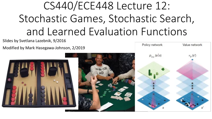
CS440/ECE448 Lecture 12: Stochastic Games, Stochastic Search, and - - PowerPoint PPT Presentation

CS440/ECE448 Lecture 12: Stochastic Games, Stochastic Search, and Learned Evaluation Functions

Slides by Svetlana Lazebnik, 9/2016 Modified by Mark Hasegawa-Johnson, 2/2019

Reminder: Exam 1 (“Midterm”) Thu, Feb 28 in class

• Review in next lecture
• Closed-book exam

(no calculators, no cheat sheets)

• Mostly short questions

Types of game environments

Deterministic Stochastic Perfect information (fully observable) Imperfect information (partially observable) Chess, checkers, go Backgammon, monopoly Battleship Scrabble, poker, bridge

Content of today’s lecture

• Stochastic games: the Expectiminimax algorithm
• Imperfect information
• Minimax formulation
• Expectiminimax formulation
• Stochastic search, even for deterministic games
• Learned evaluation functions
• Case study: Alpha-Go

Stochastic games

How can we incorporate dice throwing into the game tree?

Stochastic games

Minimax vs. Expectiminimax

• Minimax:
• Maximize (over all possible moves I can make) the
• Minimum (over all possible moves Min can make) of the
• Reward

!"#$%('()%) = max

/0 /1234

min

789:4 /1234 ;%<"=)

• Expectiminimax:
• Maximize (over all possible moves I can make) the
• Minimum (over all possible moves Min can make) of the
• Expected reward

!"#$%('()%) = max

/0 /1234

min

789:4 /1234 > ;%<"=)

> ;%<"=) = ?

1@AB1/34

C=(D"DE#EFG ($FH(I% ×;%<"=)(($FH(I%)

Stochastic games

Expectiminimax: Compute value of terminal, MAX and MIN nodes like minimax, but for CHANCE nodes, sum values of successor states weighted by the probability of each successor

• Value(node) =

§ Utility(node) if node is terminal § maxaction Value(Succ(node, action)) if type = MAX § minaction Value(Succ(node, action)) if type = MIN § sumaction P(Succ(node, action)) * Value(Succ(node, action)) if type = CHANCE

Expectiminimax example

• RANDOM: Max flips a coin. It’s heads or tails.
• MAX: Max either stops, or continues.
• Stop on heads: Game ends, Max wins (value = $2).
• Stop on tails: Game ends, Max loses (value = -$2).
• Continue: Game continues.
• RANDOM: Min flips a coin.
• HH: value = $2
• TT: value = -$2
• HT or TH: value = 0
• MIN: Min decides whether to keep the current
• utcome (value as above), or pay a penalty

(value=$1).

T H H H T T 2

• 2

2 1 1 0 1 -2 1 1

• 2

½

• 1

2

• 1

½

Expectiminimax summary

• All of the same methods are useful:
• Alpha-Beta pruning
• Evaluation function
• Quiescence search, Singular move
• Computational complexity is pretty bad
• Branching factor of the random choice can be high
• Twice as many “levels” in the tree

Games of Imperfect Information

Imperfect information example

• Min chooses a coin:
• Penny (1 cent): Lincoln
• Nickel (5 cent): Jefferson
• I say the name of a U.S. President.
• If I guessed right, she gives me the coin.
• If I guessed wrong, I have to give her a

coin to match the one she has.

1

• 5

5

• 1

Imperfect information example

• The problem: I don’t know which

state I’m in. I only know it’s one of these two

1

• 5

5

• 1

Method #1: Treat “unknown” as “random”

• Expectiminimax: treat the unknown

information as random.

• Choose the policy that maximizes

my expected reward.

• “Lincoln”:

! " ×1 + ! " × −5 = −2

• “Jefferson”:

! " ×(−1) + ! " ×5 = 2

• Expectiminimax policy: say

“Jefferson”.

• BUT WHAT IF and are not

equally likely? 1

• 5

5

• 1

Method #2: Treat “unknown” as “unknown”

• Suppose Min can choose whichever coin

she wants. She knows that I will pick Jefferson – then she will pick the penny!

• Another reasoning: I want to know what

is my worst-case outcome (e.g., to decide if I should even play this game…)

• The solution: choose the policy that

maximizes my minimum reward.

• “Lincoln”: minimum reward is -5.
• “Jefferson”: minimum reward is -1.
• Miniminimax policy: say “Jefferson”.

1

• 5

5

• 1

How to deal with imperfect information

• If you think you know the probabilities of different settings, and if

you want to maximize your average winnings (for example, you can afford to play the game many times): expectiminimax

• If you have no idea of the probabilities of different settings; or, if you

can only afford to play once, and you can’t afford to lose: miniminimax

• If the unknown information has been selected intentionally by your
• pponent: use game theory

Mi Minimi minima max with imperfect information

• Minimax:
• Maximize (over all possible moves I can make) the
• Minimum
• (over all possible states of the information I don’t know,
• … over all possible moves Min can make) the
• Reward.

!"#$%('()%) = max

/0123 45673

min

/:;23 45673

min

4:33:;< :;=5

>%?"@)

Stochastic games of imperfect information

Source States are grouped into information sets for each player

Stochastic search

Stochastic search for stochastic games

• The problem with expectiminimax: huge branching factor (many possible outcomes)

! "#$%&' = )

*+,-*./0

1&23%345467 28692:# ×"#$%&'(28692:#)

• An approximate solution: Monte Carlo search

! "#$%&' ≈ 1 @ )

ABC D

"#$%&'(4E6ℎ &%@'2: G%:#)

• Asymptotically optimal: as @ → ∞, the approximation gets better.
• Controlled computational complexity: choose n to match the amount of

computation you can afford.

Monte Carlo Tree Search

• What about deterministic games with deep trees, large branching

factor, and no good heuristics – like Go?

• Instead of depth-limited search with an evaluation function,

use randomized simulations

• Starting at the current state (root of search tree), iterate:
• Select a leaf node for expansion

using a tree policy (trading off exploration and exploitation)

• Run a simulation using

a default policy (e.g., random moves) until a terminal state is reached

• Back-propagate the outcome

to update the value estimates

• f internal tree nodes
• C. Browne et al., A survey of Monte Carlo Tree Search Methods, 2012

Monte Carlo Tree Search

Current state = root of tree Node weights: wins/total playouts for current player Leaf nodes = nodes where no simulation (”playout”) has been performed yet

• 1. Selection: Start from root (current state), select successive nodes until a leaf node L is reached
• 2. Expansion: Unless L is decisive win/loose/draw, create children for L, and choose one child C to expand
• 3. Simulation: keep choosing moves from C until game is finished
• 4. Backpropagation: update outcome of game up the tree.

Exploration vs Exploitation (briefly)

• Exploration: how much can we afford to explore the space to gather

more information?

• Exploitation: how can we maximize expected payoff (given the

information we have)

Learned evaluation functions

Stochastic search off-line

Training phase:

• Spend a few weeks allowing your computer to play

billions of random games from every possible starting state

• Value of the starting state = average value of the ending states

achieved during those billion random games Testing phase:

• During the alpha-beta search, search until you reach a state whose

value you have stored in your value lookup table

• Oops…. Why doesn’t this work?

Evaluation as a pattern recognition problem

Training phase:

• Spend a few weeks allowing your computer to play billions of random games from

billions of possible starting states.

• Value of the starting state = average value of the ending states achieved during those

billion random games Generalization:

• Featurize (e.g., x1=number of patterns, x2 = number of patterns, etc.)
• Linear regression: find a1, a2, etc. so that Value(state) ≈ a1*x1+a2*x2+…

Testing phase:

• During the alpha-beta search, search as deep as you can, then estimate the value of each

state at your horizon using Value(state) ≈ a1*x1+a2*x2+…

Pros and Cons

• Learned evaluation function
• Pro: off-line search permits lots of compute time, therefore lots of training

data

• Con: there’s no way you can evaluate every starting state that might be

achieved during actual game play. Some starting states will be missed, so generalized evaluation function is necessary

• On-line stochastic search
• Con: limited compute time
• Pro: it’s possible to estimate the value of the state you’ve reached during

actual game play

Case study: AlphaGo

• “Gentlemen

should not waste their time

• n trivial games
• - they should

play go.”

• -- Confucius,
• The Analects
• ca. 500 B. C. E.

Anton Ninno Roy Laird, Ph.D. antonninno@yahoo.com roylaird@gmail.com special thanks to Kiseido Publications

AlphaGo

• Deep convolutional

neural networks

• Treat the Go board as an

image

• Powerful function

approximation machinery

• Can be trained to predict

distribution over possible moves (policy) or expected value of position

• D. Silver et al., Mastering the Game of Go with Deep Neural Networks and Tree Search, Nature 529,

January 2016

AlphaGo

• SL policy network
• Idea: perform supervised learning (SL) to predict human moves
• Given state s, predict probability distribution over moves a, P(a|s)
• Trained on 30M positions, 57% accuracy on predicting human moves
• Also train a smaller, faster rollout policy network (24% accurate)
• RL policy network
• Idea: fine-tune policy network using reinforcement learning (RL)
• Initialize RL network to SL network
• Play two snapshots of the network against each other, update parameters

to maximize expected final outcome

• RL network wins against SL network 80% of the time, wins against open-

source Pachi Go program 85% of the time

• D. Silver et al., Mastering the Game of Go with Deep Neural Networks and Tree Search, Nature 529,

January 2016

AlphaGo

• SL policy network
• RL policy network
• Value network
• Idea: train network for position evaluation
• Given state s, estimate v(s), expected outcome of play starting with

position s and following the learned policy for both players

• Train network by minimizing mean squared error between actual and

predicted outcome

• Trained on 30M positions sampled from different self-play games
• D. Silver et al., Mastering the Game of Go with Deep Neural Networks and Tree Search, Nature 529,

January 2016

AlphaGo

• D. Silver et al., Mastering the Game of Go with Deep Neural Networks and Tree Search, Nature 529,

January 2016

AlphaGo

• Monte Carlo Tree Search
• Each edge in the search tree maintains prior probabilities P(s,a),

counts N(s,a), action values Q(s,a)

• P(s,a) comes from SL policy network
• Tree traversal policy selects actions that maximize Q value plus

exploration bonus (proportional to P but inversely proportional to N)

• An expanded leaf node gets a value estimate that is a

combination of value network estimate and outcome of simulated game using rollout network

• At the end of each simulation, Q values are updated to the

average of values of all simulations passing through that edge

• D. Silver et al., Mastering the Game of Go with Deep Neural Networks and Tree Search, Nature 529,

January 2016

AlphaGo

• Monte Carlo Tree Search
• D. Silver et al., Mastering the Game of Go with Deep Neural Networks and Tree Search, Nature 529,

January 2016

AlphaGo

• D. Silver et al., Mastering the Game of Go with Deep Neural Networks and Tree Search, Nature 529,

January 2016

Alpha-Go video

Game AI: Origins

• Minimax algorithm: Ernst Zermelo, 1912
• Chess playing with evaluation function, quiescence

search, selective search: Claude Shannon, 1949 (paper)

• Alpha-beta search: John McCarthy, 1956
• Checkers program that learns its own evaluation

function by playing against itself: Arthur Samuel, 1956 (Rodney Brooks blog post)

Game AI: State of the art

• Computers are better than humans:
• Checkers: solved in 2007
• Chess:
• State-of-the-art search-based systems now better than humans
• Deep learning machine teaches itself chess in 72 hours, plays at

International Master Level (arXiv, September 2015)

• Computers are competitive with top human players:
• Backgammon: TD-Gammon system (1992) used reinforcement

learning to learn a good evaluation function

• Bridge: top systems use Monte Carlo simulation and alpha-

beta search

• Go: computers were not considered competitive until AlphaGo

in 2016

Game AI: State of the art

• Computers are not competitive with top human players:
• Poker
• Heads-up limit hold’em poker is solved (2015)
• Simplest variant played competitively by humans
• Smaller number of states than checkers, but partial observability makes it difficult
• Essentially weakly solved = cannot be beaten with statistical significance

in a lifetime of playing

• CMU’s Libratus system beats four of the best human players at no-limit

Texas Hold’em poker (2017)

http://xkcd.com/1002/ See also: http://xkcd.com/1263/

Calvinball:

• Play it online
• Watch an instructional video