CS 440/ECE448 Lecture 19: Bayes Net Inference Mark - - PowerPoint PPT Presentation

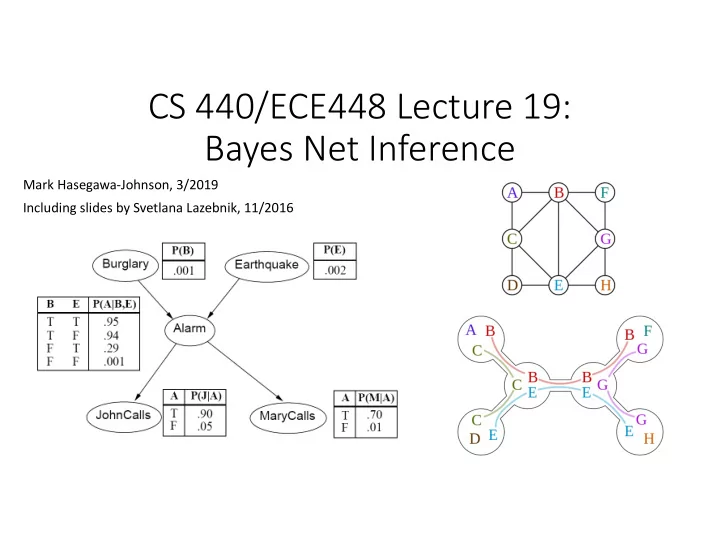
CS 440/ECE448 Lecture 19: Bayes Net Inference

Mark Hasegawa-Johnson, 3/2019 Including slides by Svetlana Lazebnik, 11/2016

Bayes Network Inference & Learning

Bayes net is a memory-efficient model of dependencies among:

• Query variables: X
• Evidence (observed) variables and their values: E = e
• Unobserved variables: Y

Inference problem: answer questions about the query variables given the evidence variables

• This can be done using the posterior distribution P(X | E = e)
• The posterior can be derived from the full joint P(X, E, Y)
• How do we make this computationally efficient?

Learning problem: given some training examples, how do we learn the parameters of the model?

• Parameters = p(variable|parents), for each variable in the net

Outline

• Inference Examples
• Inference Algorithms
• Trees: Sum-product algorithm
• Poly-trees: Junction tree algorithm
• Graphs: No polynomial-time algorithm
• Parameter Learning

Practice example 1

• Variables: Cloudy, Sprinkler, Rain, Wet Grass

Practice example 1

• Given that the grass is wet, what is the probability

that it has rained?

P(r | w) = P(r,w) P(w) = P(c,s,r,w)

C=c,S=s

∑

P(c,s,r,w)

C=c,S=s,R=r

∑

= P(c)P(s | c)P(r | c)P(w | r,s)

C=c,S=s

∑

P(c)P(s | c)P(r | c)P(w | r,s)

C=c,S=s,R=r

∑

Practice Example #2

• Suppose you have an observation, for example, “Jack called” (J=1)
• You want to know: was there a burglary?
• You need

𝑄 𝐶 = 1 𝐾 = 1 = 𝑄(𝐶, 𝐾 = 1) ∑* 𝑄(𝐶 = 𝑐, 𝐾 = 1)

• So you need to compute the table P(B,J) for all possible settings of

(B,J)

Bayes Net Inference: The Hard Way

• 1. P(B,E,A,J,M)=P(B)P(E)P(A|B,E)P(J|A)P(M|A)
• 2. 𝑄 𝐶, 𝐾 = ∑. ∑/ ∑0 𝑄(𝐶, 𝐹, 𝐵, 𝐾, 𝑁)

Exponential complexity (#P-hard, actually): N variables, each of which has K possible values ⇒ 𝑃{𝐿8} time complexity

Is there an easier way?

• Tree-structured Bayes nets: the sum-product algorithm
• Quadratic complexity, 𝑃{𝑂𝐿;}
• Polytrees: the junction tree algorithm
• Pseudo-polynomial complexity, 𝑃{𝑂𝐿0}, for M<N
• Arbitrary Bayes nets: #P complete, 𝑃{𝐿8}
• The SAT problem is a Bayes net!
• Parameter Learning

• 1. Tree-Structured Bayes Nets
• Suppose these are all binary variables.
• We observe E=1
• We want to find P(H=1|E=1)
• Means that we need to find both

P(H=0,E=1) and P(H=1,E=1) because 𝑄 𝐼 = 1 𝐹 = 1 = 𝑄(𝐼 = 1, 𝐹 = 1) ∑= 𝑄(𝐼 = ℎ, 𝐹 = 1)

The Sum-Product Algorithm (Belief Propagation)

• Find the only undirected path from the

evidence variable to the query variable (EDBFGIH)

• Find the directed root of this path P(F)
• Find the joint probabilities of root and

evidence: P(F=0,E=1) and P(F=1,E=1)

• Find the joint probabilities of query and

evidence: P(H=0,E=1) and P(H=1,E=1)

• Find the conditional probability P(H=1|E=1)

The Sum-Product Algorithm

Starting with the root P(F), we find P(F,E) by alternating product steps and sum steps:

• 1. Product: P(B,D,F)=P(F)P(B|F)P(D|B)
• 2. Sum: 𝑄 𝐸, 𝐺 = ∑ABC

D

𝑄(𝐶, 𝐸, 𝐺)

• 3. Product: P(D,E,F)=P(D,F)P(E|D)
• 4. Sum: 𝑄 𝐹, 𝐺 = ∑EBC

D

𝑄(𝐸, 𝐹, 𝐺)

The Sum-Product Algorithm (Belief Propagation)

The Sum-Product Algorithm

Starting with the root P(E,F), we find P(E,H) by alternating product steps and sum steps:

• 1. Product: P(E,F,G)=P(E,F)P(G|F)
• 2. Sum: 𝑄 𝐹, 𝐻 = ∑GBC

D

𝑄(𝐹, 𝐺, 𝐻)

• 3. Product: P(E,G,I)=P(E,G)P(I|G)
• 4. Sum: 𝑄 𝐹, 𝐽 = ∑IBC

D

𝑄(𝐹, 𝐻, 𝐽)

• 5. Product: P(E,H,I)=P(E,I)P(I|G)
• 6. Sum: 𝑄 𝐹, 𝐼 = ∑JBC

D

𝑄(𝐹, 𝐼, 𝐽)

The Sum-Product Algorithm (Belief Propagation)

• Each product step generates a table with 3

variables

• Each sum step reduces that to a table with

2 variables

• If each variable has K values, and if there

are 𝑃{𝑂} variables on the path from evidence to query, then time complexity is 𝑃{𝑂𝐿;}

Time Complexity of Belief Propagation

Time Complexity of Bayes Net Inference

• Tree-structured Bayes nets: the sum-product algorithm
• Quadratic complexity, 𝑃{𝑂𝐿;}
• Polytrees: the junction tree algorithm
• Pseudo-polynomial complexity, 𝑃{𝑂𝐿0}, for M<N
• Arbitrary Bayes nets: #P complete, 𝑃{𝐿8}
• The SAT problem is a Bayes net!
• Parameter Learning

• 2. The Junction Tree Algorithm
• a. Moralize the graph (identify each variable’s Markov blanket)
• b. Triangulate the graph (eliminate undirected cycles)
• c. Create the junction tree (form cliques)
• d. Run the sum-product algorithm on the junction tree

2.a. Markov Blanket

• Suppose there is a Bayes net

with variables A,B,C,D,E,F,G,H

• The “Markov blanket” of

variable F is D,E,G if P(F|A,B,C,D,E,G,H) = P(F|D,E,G)

2.a. Markov Blanket

• Suppose there is a Bayes net

with variables A,B,C,D,E,F,G,H

• The “Markov blanket” of

variable F is D,E,G if P(F|A,B,C,D,E,G,H) = P(F|D,E,G)

A B C D E F G H

2.a. Markov Blanket

• The “Markov blanket” of variable F is

D,E,G if P(F|A,B,C,D,E,G,H) = P(F|D,E,G)

• How can we prove that?
• P(A,…,H) = P(A)P(B|A) …
• Which of those terms include F?

A B C D E F G H

2.a. Markov Blanket

• Which of those terms include F?
• Only these two:

P(F|D) and P(G|E,F)

A B C D E F G H

2.a. Markov Blanket

The Markov Blanket of variable F includes only its immediate family members:

• Its parent, D
• Its child, G
• The other parent of its child, E

Because P(F|A,B,C,D,E,G,H) = P(F|D,E,G)

A B C D E F G H

2.a. Moralization

“Moralization” =

• 1. If two variables have a child

together, force them to get married.

• 2. Get rid of the arrows (not

necessary any more). Result: Markov blanket = the set of variables to which a variable is connected.

A B C D E F G H

2.b. Triangulation

Triangulation = draw edges so that there is no unbroken cycle of length > 3. There are usually many different ways to do this. For example, here’s one:

A B C D E F G H

2.c. Form Cliques

Clique = a group of variables, all of whom are members of each other’s immediate family. Junction Tree = a tree in which

• Each node is a clique from the
• riginal graph,
• Each edge is an “intersection set,”

naming the variables that overlap between the two cliques.

A B C D E F G H AB BCD CDF CEF EFG GH

B CD CF EF G

2.d. Sum-Product

Suppose we need P(B,G):

• 1. Product: P(B,C,D,F)=P(B)P(C|B)P(D|B)P(F|D)
• 2. Sum: 𝑄 𝐶, 𝐷, 𝐺 = ∑E 𝑄(𝐶, 𝐷, 𝐸, 𝐺)
• 3. Product: P(B,C,E,F)=P(B,C,F)P(E|C)
• 4. Sum: 𝑄 𝐶, 𝐹, 𝐺 = ∑L 𝑄(𝐶, 𝐷, 𝐹, 𝐺)
• 5. Product: P(B,E,F,G) = P(B,E,F)P(G|E,F)
• 6. Sum: 𝑄 𝐶, 𝐻 = ∑. ∑G 𝑄(𝐶, 𝐹, 𝐺, 𝐻)

Complexity: 𝑃{𝑂𝐿0}, where N=# cliques, K = # values for each variable, M = 1 + # variables in the largest clique

B C D E F G

Junction Tree: Sample Test Question

Consider the burglar alarm example.

• a. Moralize this graph
• b. Is it already triangulated? If

not, triangulate it.

• c. Draw the junction tree

Solution

• a. Moralize this graph

B E A J M

Solution

• b. Is it already triangulated?

Answer: yes. There is no unbroken cycle of length > 3.

B E A J M

Solution

• c. Draw the junction tree

ABE AJ AM

A A

Time Complexity of Bayes Net Inference

• Tree-structured Bayes nets: the sum-product algorithm
• Quadratic complexity, 𝑃{𝑂𝐿;}
• Polytrees: the junction tree algorithm
• Pseudo-polynomial complexity, 𝑃{𝑂𝐿0}, for M<N
• Arbitrary Bayes nets: #P complete, 𝑃{𝐿8}
• The SAT problem is a Bayes net!
• Parameter Learning

Bayesian network inference

• In full generality, NP-hard
• More precisely, #P-hard: equivalent to counting satisfying assignments
• We can reduce satisfiability to Bayesian network inference
• Decision problem: is P(Y) > 0?

Y = (U1 ∨U2 ∨U3)∧(¬U1 ∨¬U2 ∨U3)∧(U2 ∨¬U3 ∨U4)

Bayesian network inference

• In full generality, NP-hard
• More precisely, #P-hard: equivalent to counting satisfying assignments
• We can reduce satisfiability to Bayesian network inference
• Decision problem: is P(Y) > 0?
• G. Cooper, 1990

Y = (U1 ∨U2 ∨U3)∧(¬U1 ∨¬U2 ∨U3)∧(U2 ∨¬U3 ∨U4)

C1 C2 C3

Bayesian network inference

P(U1,U2,U3,U4,C1,C2,C3, D1, D2,Y) = P(U1)P(U2)P(U3)P(U4) P(C1 |U1,U2,U3)P(C2 |U1,U2,U3)P(C3 |U2,U3,U4) P(D1 |C1)P(D2 | D1,C2)P(Y | D2,C3)

Bayesian network inference

Why can’t we use the junction tree algorithm to efficiently compute Pr(Y)?

Bayesian network inference

Why can’t we use the junction tree algorithm to efficiently compute Pr(Y)? Answer: after we moralize and triangulate, the size of the largest clique (u2u3c1c2c3) is 𝑁 ≈ 𝑂, same order

• f magnitude as the original problem

Time Complexity of Bayes Net Inference

• Tree-structured Bayes nets: the sum-product algorithm
• Quadratic complexity, 𝑃{𝑂𝐿;}
• Polytrees: the junction tree algorithm
• Pseudo-polynomial complexity, 𝑃{𝑂𝐿0}, for M<N
• Arbitrary Bayes nets: #P complete, 𝑃{𝐿8}
• The SAT problem is a Bayes net!
• Parameter Learning

Parameter learning

• Inference problem: given values of evidence variables

E = e, answer questions about query variables X using the posterior P(X | E = e)

• Learning problem: estimate the parameters of the

probabilistic model P(X | E) given a training sample {(x1,e1), …, (xn,en)}

Parameter learning: complete data

• Suppose we know the network structure (but not the

parameters), and have a training set of complete

• bservations

Sample

C S R W 1 T F T T 2 F T F T 3 T F F F 4 T T T T 5 F T F T 6 T F T F … … … …. …

? ? ? ? ? ? ? ? ?

Training set

Parameter learning

• Suppose we know the network structure (but not the

parameters), and have a training set of complete

• bservations
• Example:

𝑄 𝑇 = 𝑈 𝐷 = 𝑈 = #samples with 𝑇 = 𝑈, 𝐷 = 𝑈 # samples with 𝐷 = 𝑈 = 1 4

Sample

C S R W 1 T F T T 2 F T F T 3 T F F F 4 T T T T 5 F T F T 6 T F T F … … … …. …

Training set

Parameter learning

• Suppose we know the network structure (but not the

parameters), and have a training set of complete

• bservations
• P(X | Parents(X)) is given by the observed frequencies of

the different values of X for each combination of parent values

Parameter learning: missing data

• Suppose we know the network structure (but not the

parameters), and have a training set, but the training set is missing some observations.

? ? ? ? ? ? ? ? ?

Training set

Sample

C S R W 1 ? F T T 2 ? T F T 3 ? F F F 4 ? T T T 5 ? T F T 6 ? F T F … … … …. …

Missing data: the EM algorithm

• The EM algorithm starts (“Expectation Maximization”)

starts with an initial guess for each parameter value.

• We try to improve the initial guess, using the algorithm on the

next two slides:

• E-step
• M-step

0.5? 0.5? 0.5? 0.5? 0.5? 0.5? 0.5? 0.5? 0.5?

Training set

Sample

C S R W 1 ? F T T 2 ? T F T 3 ? F F F 4 ? T T T 5 ? T F T 6 ? F T F … … … …. …

Missing data: the EM algorithm

• E-Step (Expectation): Given the model parameters, replace each of the missing

numbers with a probability (a number between 0 and 1) using 𝑄 𝐷 = 1 𝑇, 𝑆, 𝑋 = 𝑄(𝐷 = 1, 𝑇, 𝑆, 𝑋) 𝑄 𝐷 = 1, 𝑇, 𝑆, 𝑋 + 𝑄(𝐷 = 0, 𝑇, 𝑆, 𝑋)

0.5? 0.5? 0.5? 0.5? 0.5? 0.5? 0.5? 0.5? 0.5?

Training set

Sample

C S R W 1 0.5? F T T 2 0.5? T F T 3 0.5? F F F 4 0.5? T T T 5 0.5? T F T 6 0.5? F T F … … … …. …

Missing data: the EM algorithm

• M-Step (Maximization): Given the missing data estimates, replace each of the

missing model parameters using 𝑄 Variable = T Parents = value = 𝐹[# times Variable = 𝑈, Parents = value] 𝐹[#times Parents = value]

0.5 0.5 0.5 0.5 0.5 1.0 1.0 0.5 0.0

Training set

Sample

C S R W 1 0.5? F T T 2 0.5? T F T 3 0.5? F F F 4 0.5? T T T 5 0.5? T F T 6 0.5? F T F … … … …. …

Missing data: the EM algorithm

• Iterate back and forth between E-step and M-step until the model converges.

0.5 0.5 0.5 0.5 0.5 1.0 1.0 0.5 0.0

Training set

Sample

C S R W 1 0.5? F T T 2 0.5? T F T 3 0.5? F F F 4 0.5? T T T 5 0.5? T F T 6 0.5? F T F … … … …. …

Summary: Bayesian networks

• Structure
• Parameters
• Inference
• Learning