Cognitive Modeling Unseen Examples 2 Bayes Classifiers Lecture 14: - - PowerPoint PPT Presentation

Decision Making as Classification Bayes Classifiers Naive Bayes Classifiers

Cognitive Modeling

Lecture 14: Naive Bayes Classifiers Frank Keller

School of Informatics University of Edinburgh keller@inf.ed.ac.uk

February 19, 2006

Frank Keller Cognitive Modeling 1 Decision Making as Classification Bayes Classifiers Naive Bayes Classifiers

1 Decision Making as Classification

Decision Making Frequencies and Probabilities Unseen Examples

2 Bayes Classifiers

Bayes’ Theorem Maximum A Posteriori Maximum Likelihood Properties

3 Naive Bayes Classifiers

Parameter Estimation Properties Application to Decision Making Sparse Data Reading: Mitchell (1997: Ch. 6).

Frank Keller Cognitive Modeling 2 Decision Making as Classification Bayes Classifiers Naive Bayes Classifiers Decision Making Frequencies and Probabilities Unseen Examples

Decision Making

Bayes’ Theorem can be used to devised a general model of decision making: regard decision making as classification: given a set of attributes (the data) choose a target class (the decision); decisions are based on frequency distributions in the environment; distributions can be updated incrementally as more data becomes available (model learns from experience). General form of this model Bayes classifier. With certain simplifying assumptions: Naive Bayes classifier.

Frank Keller Cognitive Modeling 3 Decision Making as Classification Bayes Classifiers Naive Bayes Classifiers Decision Making Frequencies and Probabilities Unseen Examples

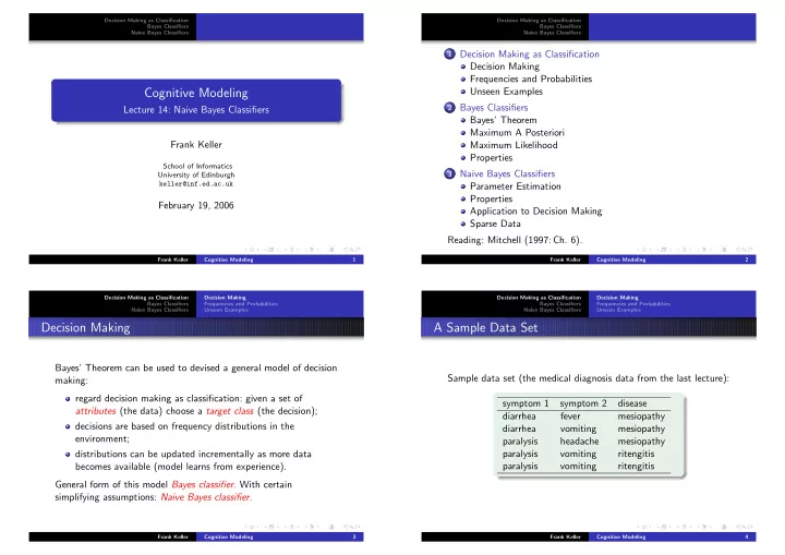
A Sample Data Set

Sample data set (the medical diagnosis data from the last lecture): symptom 1 symptom 2 disease diarrhea fever mesiopathy diarrhea vomiting mesiopathy paralysis headache mesiopathy paralysis vomiting ritengitis paralysis vomiting ritengitis

Frank Keller Cognitive Modeling 4

Decision Making as Classification Bayes Classifiers Naive Bayes Classifiers Decision Making Frequencies and Probabilities Unseen Examples

Frequencies and Probabilities

symptom 1 symptom 2 disease mes rite mes rite mes rite diarrhea 2 fever 1 3 2 paralysis 1 2 headache 1 vomiting 1 2 symptom 1 symptom 2 disease mes rite mes rite mes rite diarrhea 2/3 0/2 fever 1/3 0/2 3/5 2/5 paralysis 1/3 2/2 headache 1/3 0/2 vomiting 1/3 2/2

Frank Keller Cognitive Modeling 5 Decision Making as Classification Bayes Classifiers Naive Bayes Classifiers Decision Making Frequencies and Probabilities Unseen Examples

Classifying an Unseen Example

Now assume that we have to classify the following new instance: symptom 1 symptom 2 disease paralysis vomiting ? Key idea: compute a probability for each target class based on the probability distribution in the training data. First take into account the probability of each attribute. Treat all attributes equally important, i.e., multiply the probabilities: P(mesiopathy) = 1/3 · 1/3 = 1/9 P(ritengitis) = 2/2 · 2/2 = 1

Frank Keller Cognitive Modeling 6 Decision Making as Classification Bayes Classifiers Naive Bayes Classifiers Decision Making Frequencies and Probabilities Unseen Examples

Classifying an Unseen Example

Now take into account the overall probability of a given class. Multiply it with the probabilities of the attributes: P(mesiopathy) = 1/9 · 3/5 = 0.067 P(ritengitis) = 1 · 2/5 = 0.4 Now choose the class so that it maximizes this probability. This means that the new instance will be classified as ritengitis.

Frank Keller Cognitive Modeling 7 Decision Making as Classification Bayes Classifiers Naive Bayes Classifiers Bayes’ Theorem Maximum A Posteriori Maximum Likelihood Properties

Bayes’ Theorem

This procedure is based on Bayes’ Theorem: Bayes’ Theorem Given a hypothesis h and data D which bears on the hypothesis: P(h|D) = P(D|h)P(h) P(D) P(h): independent probability of h: prior probability P(D): independent probability of D P(D|h): conditional probability of D given h: likelihood P(h|D): conditional probability of h given D: posterior probability

Frank Keller Cognitive Modeling 8

Decision Making as Classification Bayes Classifiers Naive Bayes Classifiers Bayes’ Theorem Maximum A Posteriori Maximum Likelihood Properties

Maximum A Posteriori

Based on Bayes’ Theorem, we can compute the maximum a posteriori (MAP) hypothesis for the data: hMAP = argmax

h∈H

P(h|D) (1) = argmax

h∈H

P(D|h)P(h) P(D) = argmax

h∈H

P(D|h)P(h) H: set of all hypotheses. Note that we can drop P(D) as the probability of the data is constant (and independent of the hypothesis).

Frank Keller Cognitive Modeling 9 Decision Making as Classification Bayes Classifiers Naive Bayes Classifiers Bayes’ Theorem Maximum A Posteriori Maximum Likelihood Properties

Maximum Likelihood

Now assume that all hypotheses are equally probable a priori, i.e., P(hi) = P(hj) for all hi, hj ∈ H. This is called assuming a uniform prior. It simplifies computing the posterior: (2) hML = argmax

h∈H

P(D|h) This hypothesis is called the maximum likelihood hypothesis. It can be regarded as a model of decision making with base rate neglect.

Frank Keller Cognitive Modeling 10 Decision Making as Classification Bayes Classifiers Naive Bayes Classifiers Bayes’ Theorem Maximum A Posteriori Maximum Likelihood Properties

Properties

Bayes classifiers have the following desirable properties: Incrementality: with each training example, the prior and the likelihood can be updated dynamically: flexible and robust to errors. Combines prior knowledge and observed data: prior probability

• f a hypothesis multiplied with probability of the hypothesis

given the training data. Probabilistic hypotheses: outputs not only a classification, but a probability distribution over all classes.

Frank Keller Cognitive Modeling 11 Decision Making as Classification Bayes Classifiers Naive Bayes Classifiers Parameter Estimation Properties Application to Decision Making Sparse Data

Naive Bayes Classifiers

Assumption: training set consists of instances described as conjunctions of attributes values. The target classification based on finite set of classes V . The task of the learner is to predict the correct class for a new instance a1, a2, . . . , an. Key idea: assign most probable class vMAP using Bayes’ Theorem. vMAP = argmax

vj∈V

P(vj|a1, a2, . . . , an) (3) = argmax

vj∈V

P(a1, a2, . . . , an|vj)P(vj) P(a1, a2, . . . , an) = argmax

vj∈V

P(a1, a2, . . . , an|vj)P(vj)

Frank Keller Cognitive Modeling 12

Decision Making as Classification Bayes Classifiers Naive Bayes Classifiers Parameter Estimation Properties Application to Decision Making Sparse Data

Parameter Estimation

Estimating P(vj) is simple: compute the relative frequency of each target class in the training set. Estimating P(a1, a2, . . . , an|vj) is difficult: typically not enough instances for each attribute combination in the training set: sparse data problem. Independence assumption: attribute values are conditionally independent given the target value: naive Bayes. (4) P(a1, a2, . . . , an|vj) =

• i

P(ai|vj) Hence we get the following classifier: (5) vNB = argmax

vj∈V

P(vj)

• i

P(ai|vj)

Frank Keller Cognitive Modeling 13 Decision Making as Classification Bayes Classifiers Naive Bayes Classifiers Parameter Estimation Properties Application to Decision Making Sparse Data

Properties

Estimating P(ai|vj) instead of P(a1, a2, . . . , an|vj) greatly reduces the number of parameters (and data sparseness). The learning step in Naive Bayes consists of estimating P(ai|vj) and P(vj) based on the frequencies in the training data. An unseen instance is classified by computing the class that maximizes the posterior. When conditional independence is satisfied, Naive Bayes corresponds to MAP classification.

Frank Keller Cognitive Modeling 14 Decision Making as Classification Bayes Classifiers Naive Bayes Classifiers Parameter Estimation Properties Application to Decision Making Sparse Data

Application to Decision Making

Apply Naive Bayes to our medical data. The hypothesis space is V = {mesiopathy, ritengitis}. Classify the following instance: symptom 1 symptom 2 disease paralysis vomiting ? vNB = argmax

vj∈{mes,rite}

P(vj)

• i

P(ai|vj) = argmax

vj∈{mes,rite}

P(vj)P(sym1 = para|vj)P(sym2 = vomit|vj) Compute priors: P(disease = mes) = 3/5 P(disease = rite) = 2/5

Frank Keller Cognitive Modeling 15 Decision Making as Classification Bayes Classifiers Naive Bayes Classifiers Parameter Estimation Properties Application to Decision Making Sparse Data

Application to Decision Making

Compute conditionals (examples): P(sym1 = paralysis|disease = mes) = 1/3 P(sym1 = paralysis|disease = rite) = 2/2 Then compute the best class: P(mes)P(sym1 = paralysis|mes)P(sym2 = vomiting|disease = mes) = 3/5 · 1/3 · 1/3 = 0.067 P(rite)P(sym1 = paralysis|rite)P(sym2 = vomiting|disease = rite) = 2/5 · 2/2 · 2/2 = 0.4 Now classify the unseen instance: vNB = argmax

vj∈{mes,rite}

P(vj)P(paralysis|vj)P(vomiting|vj) = ritengitis

Frank Keller Cognitive Modeling 16

Decision Making as Classification Bayes Classifiers Naive Bayes Classifiers Parameter Estimation Properties Application to Decision Making Sparse Data

Sparse Data

Prior and conditional probabilities can be estimated from the relative frequencies in the training data: P(vj) = n N P(ai|vj) = nc n Where N is the total number of training instances; n is the total number of training instances with class vj, and nc is the number of instances with attribute ai and class vj. Problem: this provides a poor estimate if nc is very small. Extreme case: if nc = 0, then the whole posterior will be zero. Solution: smoothing: redistribute some probability mass to avoid zero probabilities.

Frank Keller Cognitive Modeling 17 Decision Making as Classification Bayes Classifiers Naive Bayes Classifiers Parameter Estimation Properties Application to Decision Making Sparse Data

Sparse Data

Smoothing technique: use the m-estimate of probabilities: P(ai|vj) = nc + mp n + m p: prior estimate of the probability m: equivalent sample size (constant) In the absence of other information, assume a uniform prior: p = 1 k where k is the number of values that the attribute ai can take.

Frank Keller Cognitive Modeling 18 Decision Making as Classification Bayes Classifiers Naive Bayes Classifiers Parameter Estimation Properties Application to Decision Making Sparse Data

Summary

We have introduced (Naive) Bayes Classifiers as a model of decision making: A Naive Bayes Classifiers can be regarded as a rational model based on Bayesian reasoning. But: does it capture the experimental data (e.g., base rate neglect and Medin and Edelson’s (1988) findings)? Naive Bayes assumes that all attributes are independent. This is clearly false in many cases. How much does this matter? Some answers to these questions will be in the assignment.

Frank Keller Cognitive Modeling 19 Decision Making as Classification Bayes Classifiers Naive Bayes Classifiers Parameter Estimation Properties Application to Decision Making Sparse Data

References

Medin, D. L. and S. M. Edelson. 1988. Problem structure and the use of base-rate information from experience. Journal of Experimental Psychology: General 117(1):68–85. Mitchell, Tom. M. 1997. Machine Learning. McGraw-Hill, New York.

Frank Keller Cognitive Modeling 20