Announcements Piazza started Matlab Grader homework, email Friday, 2 - PowerPoint PPT Presentation

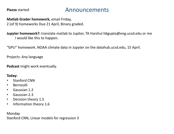
Announcements Piazza started Matlab Grader homework, email Friday, 2 (of 9) homeworks Due 21 April, Binary graded. Jupyter homework?: translate matlab to Jupiter, TA Harshul h6gupta@eng.ucsd.edu or me I would like this to happen. “GPU” homework. NOAA climate data in Jupyter on the datahub.ucsd.edu, 15 April. Projects: Any language Podcast might work eventually. Today: Stanford CNN • Bernoulli • Gaussian 1.2 • Gaussian 2.3 • Decision theory 1.5 • Information theory 1.6 • Monday Stanford CNN, Linear models for regression 3

Non-parametric method

Coin estimate (Bishop 2.1) Binary variables x={0,1} • p ( x = 1 | µ ) = µ Bernoulli distributed • Bern( x | µ ) = µ x (1 − µ ) 1 − x (2.2) E [ x ] = the Bernoulli distribution. It is easily verified that this distribution µ var[ x ] = µ (1 − µ ) . N observations, Likelihood: • | N N � � µ x n (1 − µ ) 1 − x n . p ( D| µ ) = p ( x n | µ ) = (2.5) n =1 n =1 N N � � ln p ( D| µ ) = ln p ( x n | µ ) = { x n ln µ + (1 − x n ) ln(1 − µ ) } . (2.6) n =1 n =1 Max likelihood • N µ ML = 1 � x n N n =1

Coin estimate (Bishop 2.1) Bayes p(x|y)=p(y|x)p(x) • Beta( µ | a, b ) = Γ ( a + b ) Γ ( a ) Γ ( b ) µ a − 1 (1 − µ ) b − 1 Conjugate prior • 3 3 a = 0 . 1 a = 1 b = 0 . 1 b = 1 2 2 1 1 0 0 0 0.5 1 0 0.5 1 µ µ 3 3 a = 2 a = 8 b = 3 b = 4 2 2 1 1 0 0 0 0.5 1 0 0.5 1 µ µ Bayes: 2 2 2 prior likelihood function posterior 1 1 1 0 0 0 0 0.5 1 0 0.5 1 0 0.5 1 µ µ µ

ML MAP BAYES ML point estimate • MAP point estimate (often in literature ML=MAP) • Bayes => probability =>From which all information can be obtained • – MAP, median, error estimates – Further analysis as sequential – Disadvantage… not a point estimate. 2 2 2 prior likelihood function posterior 1 1 1 0 0 0 0 0.5 1 0 0.5 1 0 0.5 1 µ µ µ

Bayes Rule P ( hypothesis | data ) = P ( data | hypothesis ) P ( hypothesis ) P ( data ) Rev’d Thomas Bayes (1702–1761) • Bayes rule tells us how to do inference about hypotheses from data. • Learning and prediction can be seen as forms of inference.

The Gaussian Distribution Gaussian Mean and Variance

Gaussian Parameter Estimation Likelihood function Maximum (Log) Likelihood

Curve Fitting Re-visited, Bishop1.2.5

Maximum Likelihood N � N � t n | y ( x n , w ) , β − 1 � p ( t | x , w , β ) = . (1.61) n =1 As we did in the case of the simple Gaussian distribution earlier, it is convenient to maximize the logarithm of the likelihood function. Substituting for the form of the Gaussian distribution, given by (1.46), we obtain the log likelihood function in the form N { y ( x n , w ) − t n } 2 + N 2 ln β − N ln p ( t | x , w , β ) = − β � 2 ln(2 π ) . (1.62) 2 n =1 Consider first the determination of the maximum likelihood solution for the polyno- N 1 = 1 { y ( x n , w ML ) − t n } 2 . � (1.63) N β ML n =1 Giving estimates of W and beta, we can predict t | y ( x, w ML ) , β − 1 p ( t | x, w ML , β ML ) = N � � . (1.64) ML take a step towards a more Bayesian approach and introduce a prior

MAP: A Step towards Bayes 1.2.5 Determine by minimizing regularized sum-of-squares error, . Regularized sum of squares

Predictive Distribution True data Estimated +/- std dev

Parametric Distributions Basic building blocks: Need to determine given Representation: or ? Recall Curve Fitting We focus on Gaussians!

The Gaussian Distribution

Central Limit Theorem • The distribution of the sum of N i.i.d. random variables becomes increasingly Gaussian as N grows. • Example: N uniform [0,1] random variables.

Geometry of the Multivariate Gaussian

Moments of the Multivariate Gaussian (2) A Gaussian requires D*(D-1)/2 +D parameters. Often we use D +D or Just D+1 parameters.

Partitioned Conditionals and Marginals, page 89

ML for the Gaussian (1) Bisphop 2.3.4 Given i.i.d. data , the log likelihood function is given by ∂ A − 1 � T ∂ A ln | A | = � (C.28) ∂ ∂ A Tr ( AB ) = B T . (C.24) ∂ = − A − 1 ∂ A � A − 1 � ∂ x A − 1 (C.21) ∂ x

Maximum Likelihood for the Gaussian Set the derivative of the log likelihood function to zero, • and solve to obtain • Similarly •

Mixtures of Gaussians (Bishop 2.3.9) Old Faithful geyser: The time between eruptions has a bimodal distribution, with the mean interval being either 65 or 91 minutes, and is dependent on the length of the prior eruption. Within a margin of error of ±10 minutes, Old Faithful will erupt either 65 minutes after an eruption lasting less than 2 1 ⁄ 2 minutes, or 91 minutes after an eruption lasting more than 2 1 ⁄ 2 minutes. Single Gaussian Mixture of two Gaussians

Mixtures of Gaussians (Bishop 2.3.9) • Combine simple models into a complex model: Component Mixing coefficient K=3

Mixtures of Gaussians (Bishop 2.3.9)

Mixtures of Gaussians (Bishop 2.3.9) Determining parameters p , µ , and S using maximum log likelihood • Log of a sum; no closed form maximum. Solution: use standard, iterative, numeric optimization methods or the • expectation maximization algorithm (Chapter 9).

Entropy 1.6 Important quantity in • coding theory • statistical physics • machine learning

Differential Entropy Put bins of width ¢ along the real line For fixed differential entropy maximized when in which case

The Kullback-Leibler Divergence P true distribution, q is approximating distribution

Decision Theory Inference step Determine either or . Decision step For given x, determine optimal t.

Minimum Misclassification Rate

• UNTIL HERE 4 April 2018

Bayes for linear model ! = #$ + & &~N(*, ,-) y ~N(#$, ,-) prior: x ~N(*, ,-) / $ ! ~/ ! $ / $ ~0 !, , /

Bayes’ Theorem for Gaussian Variables Given • we have • where •

Sequential Estimation Contribution of the N th data point, x N correction given x N correction weight old estimate

Bayesian Inference for the Gaussian Bishop2.3.6 Assume s 2 is known. Given i.i.d. data • the likelihood function for µ is given by This has a Gaussian shape as a function of µ (but it is not a distribution over µ ). •

Bayesian Inference for the Gaussian Bishop2.3.6 Combined with a Gaussian prior over µ , • this gives the posterior • Completing the square over µ , we see that •

Bayesian Inference for the Gaussian (3) Example: for N = 0, 1, 2 and 10. • Prior

Bayesian Inference for the Gaussian (4) Sequential Estimation The posterior obtained after observing N-1 data points becomes the prior when we observe the N th data point.

• NON PARAMETRIC

Nonparametric Methods (1) Parametric distribution models are restricted to specific forms, which may not • always be suitable; for example, consider modelling a multimodal distribution with a single, unimodal model. Nonparametric approaches make few assumptions about the overall shape of • the distribution being modelled. 1000 parameter versus 10 parameter •

Nonparametric Methods (2) Histogram methods partition the data space into distinct bins with widths ¢ i and count the number of observations, n i , in each bin. Often, the same width is used for • all bins, D i = D . D acts as a smoothing parameter. • In a D-dimensional space, using M • bins in each dimension will require M D bins!

Nonparametric Methods (3) If the volume of R, V, is sufficiently • Assume observations drawn from a small, p(x) is approximately density p(x) and consider a small constant over R and region R containing x such that Thus • The probability that K out of N observations lie inside R is Bin(KjN,P ) and if N is large V small, yet K>0, therefore N large?

Nonparametric Methods (4) • Kernel Density Estimation: fix V, estimate K from the data. Let R be a hypercube centred on x and define the kernel function (Parzen window) • It follows that and hence •

Nonparametric Methods (5) • To avoid discontinuities in p(x), use a smooth kernel, e.g. a Gaussian • Any kernel such that h acts as a smoother. • will work.

Nonparametric Methods (6) • Nearest Neighbour Density Estimation: fix K, estimate V from the data. Consider a hypersphere centred on x and let it grow to a volume, V ? , that includes K of the given N data points. Then K acts as a smoother.

Nonparametric Methods (7) Nonparametric models (not histograms) requires storing and computing with • the entire data set. Parametric models, once fitted, are much more efficient in terms of storage • and computation.

K-Nearest-Neighbours for Classification (1) • Given a data set with N k data points from class C k and , we have • and correspondingly • Since , Bayes’ theorem gives

K-Nearest-Neighbours for Classification (2) K = 1 K = 3