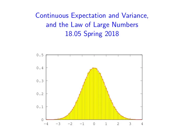
Continuous Expectation and Variance, and the Law of Large Numbers - PowerPoint PPT Presentation

Continuous Expectation and Variance, and the Law of Large Numbers 18.05 Spring 2018 0.5 0.4 0.3 0.2 0.1 0 -4 -3 -2 -1 0 1 2 3 4

Recall Exponential Random Variables Parameter: λ (called the rate parameter). Range: [0 , ∞ ). Expected value: 1 /λ Notation: exponential( λ ) or exp( λ ). f ( x ) = λ e − λ x for 0 ≤ x . Density: Models: Waiting time. large rate ↔ large λ ↔ small wait. f ( x ) = λ e − λx λ x 2 4 6 8 10 12 14 16 Continuous analogue of geometric distribution—memoryless! February 26, 2018 2 / 21

Board question I’ve noticed that taxis drive past 77 Mass. Ave. once every 10 minutes on average. Suppose time spent waiting for a taxi is modeled by an exponential random variable f ( x ) = 1 10 e − x / 10 X ∼ Exponential(1 / 10); (a) Sketch the pdf of this distribution (b) Shade the region which represents the probability of waiting between 3 and 7 minutes (c) Compute the probability of waiting between between 3 and 7 minutes for a taxi (d) Compute and sketch the cdf. February 26, 2018 3 / 21

Solution Sketches for (a), (b), (d) P (3 < X < 7) .1 f ( x ) = λ e − λx x 2 4 6 8 10 12 14 16 F ( x ) = 1 − e − x/ 10 1 x 2 4 6 8 10 12 14 16 (c) � 7 1 e − x / 10 dx = − e − x / 10 � 7 February 26, 2018 4 / 21 = e − 3 / 10 − e − 7 / 10 ≈ 0 . 244 (3 < X < 7) = � �

Expected value Expected value: measure of location X continuous with range [ a , b ] and pdf f ( x ): � b E ( X ) = xf ( x ) dx . a X discrete with values x 1 , . . . , x n and pmf p ( x i ): n � E ( X ) = x i p ( x i ) . i =1 View these as essentially the same formulas. February 26, 2018 5 / 21

Variance and standard deviation Standard deviation: measure of spread, scale For any random variable X with mean µ Var( X ) = E (( X − µ ) 2 ) , � σ = Var( X ) X continuous with range [ a , b ] and pdf f ( x ): � b ( x − µ ) 2 f ( x ) dx . Var( X ) = a X discrete with values x 1 , . . . , x n and pmf p ( x i ): n � ( x i − µ ) 2 p ( x i ) . Var( X ) = i =1 View these as essentially the same formulas. February 26, 2018 6 / 21

Properties Properties: (the same for discrete and continuous) 1. E ( X + Y ) = E ( X ) + E ( Y ). 2. E ( aX + b ) = aE ( X ) + b . 3. If X and Y are independent then Var( X + Y ) = Var( X ) + Var( Y ). 4. Var( aX + b ) = a 2 Var( X ). 5. Var( X ) = E ( X 2 ) − E ( X ) 2 . February 26, 2018 7 / 21

Board question The random variable X has range [0,1] and pdf cx 2 . (a) Find c . (b) Find the mean, variance and standard deviation of X . (c) Find the median value of X . (d) Suppose X 1 , . . . X 16 are independent identically-distributed copies of X . Let X be their average. What is the standard deviation of X ? answer: See next slides. February 26, 2018 8 / 21

Solution � 1 cx 2 dx = 1 ⇒ (a) Total probability is 1: c = 3 . 0 � 1 0 3 x 3 dx = 3 / 4. (b) µ = � 1 σ 2 = ( 0 ( x − 3 / 4) 2 3 x 2 dx ) = 3 5 − 9 8 + 9 16 = 3 80 . � 3 / 80 = 1 � σ = 3 / 5 ≈ . 194 4 � x 3 u 2 du = x 3 . Therefore, (c) Set F ( q 0 . 5 ) = 0 . 5, solve for q 0 . 5 : F ( x ) = 0 0 . 5 = . 5. We get, q 0 . 5 = (0 . 5) 1 / 3 . F ( q 0 . 5 ) = q 3 (d) Because they are independent Var( X 1 + . . . + X 16 ) = Var( X 1 ) + Var( X 2 ) + . . . + Var( X 16 ) = 16Var( X ). . Finally, σ X = σ X Thus, Var( X ) = 16Var( X ) = Var( X ) 4 = 0 . 194 / 4 . 16 2 16 February 26, 2018 9 / 21

Quantiles: a measure of location φ ( z ) left tail area = prob. = .6 z q 0 . 6 = 0 . 253 Φ( z ) 1 F ( q 0 . 6 ) = 0 . 6 z q 0 . 6 = 0 . 253 q 0 . 6 : left tail area = 0.6 ⇔ F ( q 0 . 6 ) = 0 . 6 February 26, 2018 10 / 21

Concept question Each of the curves is the density for a given random variable. The median of the black plot is always at q . Which density has the greatest median? 1. Black 2. Red 3. Blue 4. All the same 5. Impossible to tell (A) (B) Curves coincide to here. q q answer: See next frame. February 26, 2018 11 / 21

Solution (A) Curves coincide to here. Area to the left of the me- dian = 0.5 q Plot A: 4. All three medians are the same. Remember that probability is computed as the area under the curve. By definition the median q is the point where the shaded area in Plot A .5. Since all three curves coincide up to q . That is, the shaded area in the figure is represents a probability of .5 for all three densities. Continued on next slide. February 26, 2018 12 / 21

Solution continued (B) q Plot B: 2. The red density has the greatest median. Since q is the median for the black density, the shaded area in Plot B is .5. Therefore the area under the blue curve (up to q ) is greater than .5 and that under the red curve is less than .5. This means the median of the blue density is to the left of q (you need less area) and the median of the red density is to the right of q (you need more area). February 26, 2018 13 / 21

Law of Large Numbers (LoLN) Informally: An average of many measurements is more accurate than a single measurement. Formally: Let X 1 , X 2 , . . . be i.i.d. random variables all with mean µ and standard deviation σ . Let n X n = X 1 + X 2 + . . . + X n = 1 � X i . n n i =1 Then for any (small number) a , we have n →∞ P ( | X n − µ | < a ) = 1 . lim No guarantees but: By choosing n large enough we can make X n as close as we want to µ with probability close to 1. February 26, 2018 14 / 21

Concept Question: Desperation You have $100. You need $1000 by tomorrow morning. Your only way to get it is to gamble. If you bet $k, you either win $k with probability p or lose $k with probability 1 − p . Maximal strategy: Bet as much as you can, up to what you need, each time. Minimal strategy: Make a small bet, say $5, each time. 1. If p = 0 . 45, which is the better strategy? (a) Maximal (b) Minimal (c) They are the same February 26, 2018 15 / 21

Concept Question: Desperation You have $100. You need $1000 by tomorrow morning. Your only way to get it is to gamble. If you bet $k, you either win $k with probability p or lose $k with probability 1 − p . Maximal strategy: Bet as much as you can, up to what you need, each time. Minimal strategy: Make a small bet, say $5, each time. 1. If p = 0 . 45, which is the better strategy? (a) Maximal (b) Minimal (c) They are the same 2. If p = 0 . 8, which is the better strategy? (a) Maximal (b) Minimal (c) They are the same answer: On next slide February 26, 2018 15 / 21

Solution to previous two problems answer: If p = 0 . 45 use maximal strategy; If p = 0 . 8 use minimal strategy. If you use the minimal strategy the law of large numbers says your average winnings per bet will almost certainly be the expected winnings of one bet. The two tables represent p = 0 . 45 and p = 0 . 8 respectively. Win -10 10 Win -10 10 0.55 0.45 0.2 0.8 p p The expected value of a $5 bet when p = 0 . 45 is -$0.50 Since on average you will lose $0.50 per bet you want to avoid making a lot of bets. You go for broke and hope to win big a few times in a row. It’s not very likely, but the maximal strategy is your best bet. The expected value when p = 0 . 8 is $3. Since this is positive you’d like to make a lot of bets and let the law of large numbers (practically) guarantee you will win an average of $6 per bet. So you use the minimal strategy. February 26, 2018 16 / 21

Histograms Made by ‘binning’ data. Frequency : height of bar over bin = number of data points in bin. Density : area of bar is the fraction of all data points that lie in the bin. So, total area is 1. frequency density 4 0.8 3 0.6 2 0.4 1 0.2 x x 0.25 0.75 1.25 1.75 2.25 0.25 0.75 1.25 1.75 2.25 Check that the total area of the histogram on the right is 1. February 26, 2018 17 / 21

Board question 1. Make both a frequency and density histogram from the data below. Use bins of width 0.5 starting at 0. The bins should be right closed. 1 1.2 1.3 1.6 1.6 2.1 2.2 2.6 2.7 3.1 3.2 3.4 3.8 3.9 3.9 2. Same question using unequal width bins with edges 0, 1, 3, 4. 3. For question 2, why does the density histogram give a more reasonable representation of the data? February 26, 2018 18 / 21

Solution 3.0 0.4 Frequency Density 2.0 0.2 1.0 0.0 0.0 0 1 2 3 4 0 1 2 3 4 Histograms with equal width bins 0.4 8 Frequency Density 6 0.2 4 2 0.0 0 0 1 2 3 4 0 1 2 3 4 Histograms with unequal width bins February 26, 2018 19 / 21

LoLN and histograms LoLN implies density histogram converges to pdf: 0.5 0.4 0.3 0.2 0.1 0 -4 -3 -2 -1 0 1 2 3 4 Histogram with bin width 0.1 showing 100000 draws from a standard normal distribution. Standard normal pdf is overlaid in red. February 26, 2018 20 / 21

Standardization Random variable X with mean µ and standard deviation σ . Y = X − µ Standardization: . σ Y has mean 0 and standard deviation 1. Standardizing any normal random variable produces the standard normal. If X ≈ normal then standardized X ≈ stand. normal. We reserve Z to mean a standard normal random variable. February 26, 2018 21 / 21