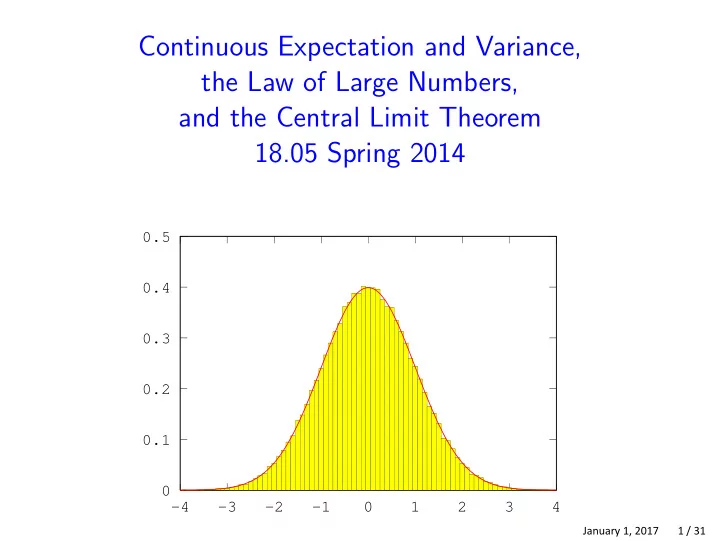
Continuous Expectation and Variance, the Law of Large Numbers, and - PowerPoint PPT Presentation

Continuous Expectation and Variance, the Law of Large Numbers, and the Central Limit Theorem 18.05 Spring 2014 0.5 0.4 0.3 0.2 0.1 0 -4 -3 -2 -1 0 1 2 3 4 January 1, 2017 1 / 31

Expected value Expected value: measure of location, central tendency X continuous with range [ a , b ] and pdf f ( x ): � b E ( X ) = xf ( x ) dx . a X discrete with values x 1 , . . . , x n and pmf p ( x i ): n n E ( X ) = x i p ( x i ) . i =1 View these as essentially the same formulas. January 1, 2017 2 / 31

Variance and standard deviation Standard deviation: measure of spread, scale For any random variable X with mean µ Var( X ) = E (( X − µ ) 2 ) , σ = Var( X ) X continuous with range [ a , b ] and pdf f ( x ): b � ( x − µ ) 2 f ( x ) dx . Var( X ) = a X discrete with values x 1 , . . . , x n and pmf p ( x i ): n n ( x i − µ ) 2 p ( x i ) . Var( X ) = i =1 View these as essentially the same formulas. January 1, 2017 3 / 31

Properties Properties: (the same for discrete and continuous) 1. E ( X + Y ) = E ( X ) + E ( Y ). 2. E ( aX + b ) = aE ( X ) + b . 3. If X and Y are independent then Var( X + Y ) = Var( X ) + Var( Y ). 4. Var( aX + b ) = a 2 Var( X ). 2 ) − E ( X ) 2 . 5. Var( X ) = E ( X January 1, 2017 4 / 31

Board question 2 The random variable X has range [0,1] and pdf cx . (a) Find c . (b) Find the mean, variance and standard deviation of X . (c) Find the median value of X . (d) Suppose X 1 , . . . X 16 are independent identically-distributed copies of X . Let X be their average. What is the standard deviation of X ? 4 . Find the pdf of Y . (e) Suppose Y = X answer: See next slides. January 1, 2017 5 / 31

Solution 1 � � 2 dx = 1 ⇒ c = 3 . (a) Total probability is 1: cx 0 1 3 x 3 dx = 3 / 4. (b) µ = 0 1 σ 2 = ( ( x − 3 / 4) 2 3 x 2 dx ) = 3 − 9 + 9 3 = 80 . 0 5 8 16 3 / 80 = 1 σ = 3 / 5 ≈ . 194 4 x � � 2 du = x . Therefore, 3 (c) Set F ( q 0 . 5 ) = 0 . 5, solve for q 0 . 5 : F ( x ) = 3 u 0 F ( q 0 . 5 ) = q 3 = . 5. We get, q 0 . 5 = (0 . 5) 1 / 3 . 0 . 5 (d) Because they are independent Var( X 1 + . . . + X 16 ) = Var( X 1 ) + Var( X 2 ) + . . . + Var( X 16 ) = 16Var( X ). σ X 16Var( X ) Var( X ) Thus, Var( X ) = = . Finally, σ = = 0 . 194 / 4 . 16 2 16 X 4 January 1, 2017 6 / 31

Solution continued (e) Method 1 use the cdf: 1 1 3 4 < y ) = P ( X < y 4 ) = F X ( y 4 ) = y 4 . F Y ( y ) = P ( X 3 − 1 � ( y ) = Now differentiate. f Y ( y ) = F y . 4 Y 4 Method 2 use the pdf: We have dy 4 3 dx ⇒ y = x ⇒ dy = 4 x = dx 3 / 4 4 y 3 y 2 / 4 dy 3 dy 1 / 4 ) This implies f X ( x ) dx = f X ( y = = dy 3 / 4 3 / 4 1 / 4 4 y 4 y 4 y 3 Therefore f Y ( y ) = 1 / 4 4 y January 1, 2017 7 / 31

Quantiles Quantiles give a measure of location. φ ( z ) left tail area = prob. = .6 z q 0 . 6 = 0 . 253 Φ( z ) 1 F ( q 0 . 6 ) = 0 . 6 z q 0 . 6 = 0 . 253 q 0 . 6 : left tail area = 0.6 ⇔ F ( q 0 . 6 ) = 0 . 6 January 1, 2017 8 / 31

Concept question Each of the curves is the density for a given random variable. The median of the black plot is always at q . Which density has the greatest median? 1. Black 2. Red 3. Blue 4. All the same 5. Impossible to tell (A) (B) Curves coincide to here. q q answer: See next frame. January 1, 2017 9 / 31

Solution (A) Curves coincide to here. Area to the left of the me- dian = 0.5 q Plot A: 4. All three medians are the same. Remember that probability is computed as the area under the curve. By definition the median q is the point where the shaded area in Plot A .5. Since all three curves coincide up to q . That is, the shaded area in the figure is represents a probability of .5 for all three densities. Continued on next slide. January 1, 2017 10 / 31

Solution continued (B) q Plot B: 2. The red density has the greatest median. Since q is the median for the black density, the shaded area in Plot B is .5. Therefore the area under the blue curve (up to q ) is greater than .5 and that under the red curve is less than .5. This means the median of the blue density is to the left of q (you need less area) and the median of the red density is to the right of q (you need more area). January 1, 2017 11 / 31

Law of Large Numbers (LoLN) Informally: An average of many measurements is more accurate than a single measurement. Formally: Let X 1 , X 2 , . . . be i.i.d. random variables all with mean µ and standard deviation σ . Let n X 1 + X 2 + . . . + X n 1 n X n = = X i . n n i =1 Then for any (small number) a , we have lim P ( | X n − µ | < a ) = 1 . n →∞ No guarantees but: By choosing n large enough we can make X n as close as we want to µ with probability close to 1. January 1, 2017 12 / 31

Concept Question: Desperation You have $100. You need $1000 by tomorrow morning. Your only way to get it is to gamble. If you bet $k, you either win $k with probability p or lose $k with probability 1 − p . Maximal strategy: Bet as much as you can, up to what you need, each time. Minimal strategy: Make a small bet, say $5, each time. 1. If p = 0 . 45, which is the better strategy? (a) Maximal (b) Minimal (c) They are the same 2. If p = 0 . 8, which is the better strategy? (a) Maximal (b) Minimal (c) They are the same answer: On next slide January 1, 2017 13 / 31

Solution to previous two problems answer: If p = 0 . 45 use maximal strategy; If p = 0 . 8 use minimal strategy. If you use the minimal strategy the law of large numbers says your average winnings per bet will almost certainly be the expected winnings of one bet. The two tables represent p = 0 . 45 and p = 0 . 8 respectively. Win -10 10 Win -10 10 0.55 0.45 0.2 0.8 p p The expected value of a $5 bet when p = 0 . 45 is -$0.50 Since on average you will lose $0.50 per bet you want to avoid making a lot of bets. You go for broke and hope to win big a few times in a row. It’s not very likely, but the maximal strategy is your best bet. The expected value when p = 0 . 8 is $3. Since this is positive you’d like to make a lot of bets and let the law of large numbers (practically) guarantee you will win an average of $6 per bet. So you use the minimal strategy. January 1, 2017 14 / 31

Histograms Made by ‘binning’ data. Frequency : height of bar over bin = number of data points in bin. Density : area of bar is the fraction of all data points that lie in the bin. So, total area is 1. frequency density 4 0.8 3 0.6 2 0.4 1 0.2 x x 0.25 0.75 1.25 1.75 2.25 0.25 0.75 1.25 1.75 2.25 Check that the total area of the histogram on the right is 1. January 1, 2017 15 / 31

Board question 1. Make both a frequency and density histogram from the data below. Use bins of width 0.5 starting at 0. The bins should be right closed. 1 1.2 1.3 1.6 1.6 2.1 2.2 2.6 2.7 3.1 3.2 3.4 3.8 3.9 3.9 2. Same question using unequal width bins with edges 0, 1, 3, 4. 3. For question 2, why does the density histogram give a more reasonable representation of the data. January 1, 2017 16 / 31

Solution 3.0 0.4 Frequency Density 2.0 0.2 1.0 0.0 0.0 0 1 2 3 4 0 1 2 3 4 Histograms with equal width bins 0.4 8 Frequency Density 6 0.2 4 2 0.0 0 0 1 2 3 4 0 1 2 3 4 Histograms with unequal width bins January 1, 2017 17 / 31

LoLN and histograms LoLN implies density histogram converges to pdf: 0.5 0.4 0.3 0.2 0.1 0 -4 -3 -2 -1 0 1 2 3 4 Histogram with bin width 0.1 showing 100000 draws from a standard normal distribution. Standard normal pdf is overlaid in red. January 1, 2017 18 / 31

Standardization Random variable X with mean µ and standard deviation σ . X − µ Standardization: Y = . σ Y has mean 0 and standard deviation 1. Standardizing any normal random variable produces the standard normal. If X ≈ normal then standardized X ≈ stand. normal. We use reserve Z to mean a standard normal random variable. January 1, 2017 19 / 31

Concept Question: Standard Normal within 1 · σ ≈ 68% Normal PDF within 2 · σ ≈ 95% within 3 · σ ≈ 99% 68% 95% 99% z σ − σ − 3 σ − 2 σ 2 σ 3 σ 1 . P ( − 1 < Z < 1) is (a) 0.025 (b) 0.16 (c) 0.68 (d) 0.84 (e) 0.95 2. P ( Z > 2) (a) 0.025 (b) 0.16 (c) 0.68 (d) 0.84 (e) 0.95 answer: 1c, 2a January 1, 2017 20 / 31

Central Limit Theorem Setting: X 1 , X 2 , . . . i.i.d. with mean µ and standard dev. σ . For each n : 1 X n = ( X 1 + X 2 + . . . + X n ) average n S n = X 1 + X 2 + . . . + X n sum . Conclusion: For large n : σ 2 � � X n ≈ N µ, n S n ≈ N n µ, n σ 2 Standardized S n or X n ≈ N(0 , 1) S n − n µ X n − µ √ √ That is, = ≈ N(0 , 1) . n σ σ/ n January 1, 2017 21 / 31

CLT: pictures Standardized average of n i.i.d. uniform random variables with n = 1 , 2 , 4 , 12. 0.4 0.5 0.35 0.4 0.3 0.25 0.3 0.2 0.2 0.15 0.1 0.1 0.05 0 0 -3 -2 -1 0 1 2 3 -3 -2 -1 0 1 2 3 0.4 0.4 0.35 0.35 0.3 0.3 0.25 0.25 0.2 0.2 0.15 0.15 0.1 0.1 0.05 0.05 0 0 -3 -2 -1 0 1 2 3 -3 -2 -1 0 1 2 3 January 1, 2017 22 / 31

CLT: pictures 2 The standardized average of n i.i.d. exponential random variables with n = 1 , 2 , 8 , 64. 1 0.7 0.6 0.8 0.5 0.6 0.4 0.3 0.4 0.2 0.2 0.1 0 0 -3 -2 -1 0 1 2 3 -3 -2 -1 0 1 2 3 0.5 0.5 0.4 0.4 0.3 0.3 0.2 0.2 0.1 0.1 0 0 -3 -2 -1 0 1 2 3 -3 -2 -1 0 1 2 3 January 1, 2017 23 / 31